Test the effect of self-consistent potentials on EXAFS analysis
Feff testing framework
Table of Contents
1 Background
In a recent post to the Ifeffit mailing list, a poor soul made this comment:
I wondering about the availability to use a newer FEFF version in Demeter. Since my knowledge only I can run FEFF6. In my case I found different discrepancies using FEFF6 and FEFF9 in the determination of bond length distances for instance. In terms of review of papers, reviewers ask to use a newer version instead FEFF6.
This is a topic that comes up regularly on the mailing list. I have, on occasion, joked that Feff9 must be 50% better than Feff6 because 9 is 50% bigger than 6.
Sadly for me, my oh-so-extraordinary wit doesn’t win a science argument. Since actual science wins science arguments, I decided to investigate the effect of different theory models on EXAFS analysis. I am doing so in the form of a set of tools published as a GitHub repository. In this way, anyone can download the tools and rerun the tests. Even better, anyone can apply the tools to new materials or new ways of computing the theory.
Because Feff9 is not freely available and redistributable, it is hard to make use of it in the manner of this exercise. Consequently, the forms of Feff used here are the two redistributable versions: the Feff6 that comes with Ifeffit and feff85exafs.
I presented these results at a recent symposium on theoretical spectroscopy. By far, the most illuminating comment was from Alexei Ankudinov, the principle author of Feff8. Alex was surprised that anyone expected Feff8 or Feff9 to make a difference for EXAFS analysis. Most of the features in those later versions, and particularly in Feff9, pertain to calculations of other spectroscopies. Other new additions to the code would not be expected to have much impact for photoelectrons of high kinetic energy, i.e. far from the absorption edge.
This page is about EXAFS analysis, not XANES calculations or calculations of other spectroscopies. Obviously, any calculation of a spectroscopy for which the photoelectron has low kinetic energy will be extremely sensitive to the details of the potential surface. Self-consistency and charge transfer are unambiguously important for such calculations. The question here is about the impact on the analysis of the EXAFS spectrum.
Be all that as it may, the “Feff8/Feff9 must be better” comment is perennial. This is my attempt to address that question with some kind of rigorous effort.
Here are the conditions of the tests:
- All XAS data were processed sensibly in Athena with E0 chosen to be the first peak of the first derivative in μ(E). That may not be the best choice of E0 in all cases, but it is the obvious first choice and the likeliest choice to be made by a novice user of the software.
- All EXAFS data were Fourier transformed starting at 3/Å and ending at a reasonable place where the signal was still much bigger than the noise. The choice of 3/Å as the starting point was deliberate. The Autobk algorithm (and, indeed, all other algorithms) is often unreliable below about 3/Å due to the fact that the μ(E) is changing very quickly in that region. Thus the data above 3/Å are likely to be reliably free of systematic error due to the details of the background removal.
- All the materials considered have well-known structures. For these tests, I want to avoid the situation where error in a fitting model could be attributed to incomplete prior knowledge about the structure. That is, I want to isolate the details of the fitting model from the details of the theoretical calculation.
- The first three examples are dense, crystalline solids for which one expects self-consistency to contribute rather little to the analysis. The remaining materials all contribute interesting features for which self-consistency and charge transfer might play a role.
- In the plots, the ranges of the Fourier transform and of the fit are indicated by vertical black lines.
- Each material is fitted using theory from the version of Feff6 that ships with Ifeffit, from feff85exafs with self-consistency turned off, and from with feff85exafs with self-consistency. In each case, the default self-energy model (Hedin-Lundqvist) was used.
- For each material that is not a molecule, the analysis is done with a sequence of self-consistency radii. This is done to test the importance of the consideration of that parameter on the analysis. In the case of hydrated uranyl hydrate, this is a molecule, but the Feff calculation is made on a crystalline analogue to the molecule. The effect of self-consistency radius is tested in that case.
- Where appropriate (bromoadamantane, for example),
the
lfmsparameter of theSCFcard is set to 1. - The uranyl calculation was a bit challenging with feff85exafs. To get the program to run to completion, it was necessary to set the FOLP parameter to 0.9 for each unique potential. Given that the quality of the fit was much the same as for using Feff6, this was not examined further. Still, this merits further attention for this material.
- I was interested to know if the effect of SCF on EXAFS fitting was different for a first shell fit as compared to a more extensive fitting model. So fits were generated for the first shells only of all materials except for uranyl hydrate for which the axial and equatorial scatterers cannot be isolated. Also, Matt tells me that, years ago, he and John looked at some Feff6/Feff8 comparisons, but only for first shell fits. These first shell fits are intended for comparison to that older work. (The results of the first shell fits are included in the repository, but not on this page as they do not tell a different story from the more complete fits presented here.)
- All fits were performed with a toolset written by Bruce and included here in this repository using the XAS analysis capabilities of Larch.
- All uncertainties are 1σ error bars determined from the diagonal elements of the covariance matrix evaluated during the Levenberg-Marquardt minimizations.
- The plots shown below for each material were generated using the tools in this repository. You will notice that they appear to be highly repetitive. For each material it is the case that the fits using the different theoretical models are nearly indistinguishable by eye. The full complement of fits are shown for the sake of completeness. As you scroll through the plots of the fit results, you may be tempted to think that the same image has been replicated several times. I assure you that each plot is actual plot made using the actual fit to the different theory models!
- The very astute Feff user might point out that the path indexing
is not guaranteed to be consistent across versions. That is, a
small MS path may barely exceed the heap criterion in one version
of Feff, but not in another. That would change the indexing for
all paths with longer half-path-lengths, thus confounding the use
of single Larch fitting script with the different version of the
theory. To avoid this problem, the pathfinder in Feff6 was run,
generating a
paths.datfile. Thispaths.datwas then copied into the folders where the various feff85exafs calculations were run. The pathfinder was then skipped in each of the Feff8 runs. This guaranteed that each theory calculation generated the same list offeffNNNN.datfiles with the same indexing. - For each material, a table of charge transfer and threshold energies is presented. This is information gleaned from Feff8’s screen messages and Feff6’s standard header. The charge transfer values are the final charge transferred for each unique potential as reported in the final round of the self-consistency loop. The threshold energy μ is reported for each self-consistency radius as well as for Feff8 without self-consistency and for Feff6. This table is included ion hopes that it will help make sense of the fitted values for E0.
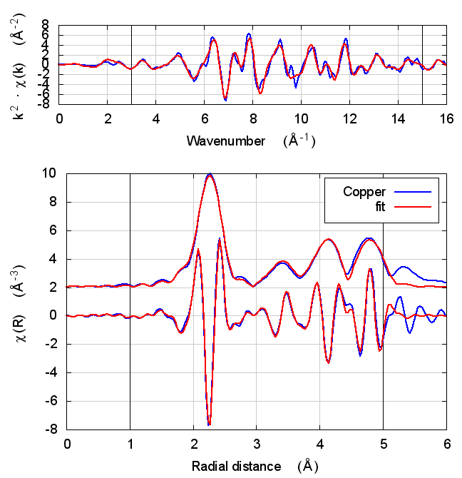
2 Copper
The data is the canonical copper foil spectrum of Newville, PhD thesis
fame. The fitting model is very simple. There is an S0² parameter
(amp), an energy shift for all paths (enot), and a volumetric
lattice expansion coefficient (alpha). The σ² values for all paths
were computed using the correlated Debye model and a temperature of
10K, except for the first shell, which has its own σ² variable
(ss1).
The fit included 4 coordination shells, which includes several co-linear multiple scattering paths of the same distance as the fourth shell single scattering path.
amp and alpha are unitless. enot is eV, ss1 is Ų, and thetad
is K.
2.1 Best fit values
| model | alpha | amp | enot | ss1 | thetad |
|---|---|---|---|---|---|
| feff6 | -0.00074(92) | 0.96(4) | 4.97(49) | 0.00382(33) | 253(22) |
| noSCF | -0.00046(90) | 0.95(4) | 5.71(48) | 0.00400(33) | 239(19) |
| withSCF(3) | -0.00077(104) | 0.94(5) | 3.45(56) | 0.00402(38) | 241(22) |
| withSCF(4) | -0.00076(104) | 0.94(5) | 3.54(56) | 0.00402(38) | 242(22) |
| withSCF(5) | -0.00077(104) | 0.94(5) | 3.40(56) | 0.00402(38) | 241(22) |
| withSCF(5.5) | -0.00077(105) | 0.94(5) | 3.41(56) | 0.00402(38) | 241(22) |
| withSCF(6) | -0.00076(104) | 0.94(5) | 3.46(56) | 0.00402(38) | 241(22) |
2.2 Statistics
| model | χ² | reduced χ² | R-factor |
|---|---|---|---|
| feff6 | 1444.2957 | 54.3832 | 0.0145 |
| noSCF | 1414.0154 | 53.2430 | 0.0142 |
| withSCF(3) | 1820.7826 | 68.5594 | 0.0182 |
| withSCF(4) | 1814.3186 | 68.3160 | 0.0182 |
| withSCF(5) | 1816.7825 | 68.4088 | 0.0182 |
| withSCF(5.5) | 1823.5990 | 68.6654 | 0.0183 |
| withSCF(6) | 1819.3955 | 68.5071 | 0.0182 |
2.3 Charge transfer and threshold energy
| ip | R=3 | R=4 | R=5 | R=5.5 | R=6 |
|---|---|---|---|---|---|
| 0 | -0.527 | -0.524 | -0.512 | -0.523 | -0.516 |
| 1 | 0.005 | 0.005 | 0.005 | 0.005 | 0.005 |
| μ | -8.091 | -7.964 | -8.104 | -8.124 | -8.056 |
Starting value for μ in feff8 = -3.820
Value for μ in feff6 = -5.519
2.4 Fits
| feff6 | no SCF | SCF, R=3 | SCF, R=4 | SCF, R=5 | SCF, R=5.5 | SCF, R=6 |
|---|---|---|---|---|---|---|
 |
 |
 |
 |
 |
 |
 |
2.5 Discussion
I start with copper because, well, because copper. All discussions of XAS theory start with copper. It’s tradition!
In fact, I expect copper to be a null result. There is no reason to expect that charge transfer and self-consistency would have much effect on a monoatomic material. That expectation is borne out.
The fitting parameters are constant well within their uncertainties and across all theory models. The statistical parameters also do not change much across the models. Amusingly, reduced χ² and R-factor are a bit smaller without the use of self-consistency.
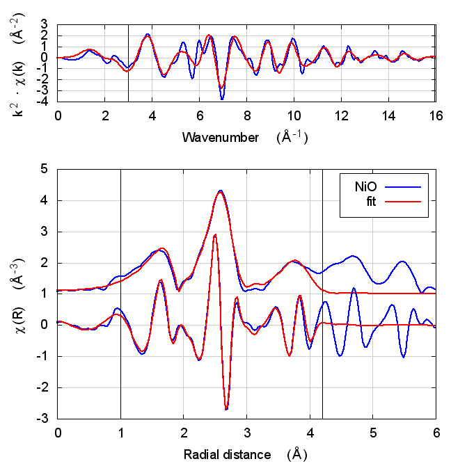
3 NiO
The sample was NiO powder prepared by my colleague Neil Hyatt
(University of Sheffield) and checked by him for phase purity. The
powder was mixed with polyethylene glycol and pressed into a pellet to
make a edge step of 0.78. The data were measured by Bruce at NSLS
beamline X23A2 and reported in a recent issue of Journal of
Synchrotron Radiation: DOI: 10.1107/S1600577515013521. The simple
fitting model to this rock salt structure included a S0² parameter
(amp), an energy shift (enot), and a volumetric lattice expansion
coefficient (alpha).
The fit included 4 coordination shells, 2 with O and 2 with Ni. There
are several co-linear multiple scattering paths at the same distance as
the fourth shell Ni scatterer. Each shell has its own σ² parameter
(sso, ssni, sso2, and ssni2, respectively.).
amp and alpha are unitless. enot is eV. sso, ssni, sso2, and
ssni2 are Ų.
3.1 Best fit values
| model | alpha | amp | enot | ssni | ssni2 | sso | sso2 |
|---|---|---|---|---|---|---|---|
| feff6 | 0.00062(146) | 0.71(5) | -1.22(54) | 0.00546(56) | 0.00714(95) | 0.00437(120) | 0.04205(3218) |
| noSCF | 0.00050(152) | 0.68(5) | 2.49(56) | 0.00534(58) | 0.00715(101) | 0.00468(131) | 0.03946(2918) |
| withSCF(2.5) | -0.00021(148) | 0.71(4) | -7.34(54) | 0.00554(56) | 0.00726(97) | 0.00468(123) | 0.03146(2038) |
| withSCF(3) | -0.00073(145) | 0.71(4) | -7.95(53) | 0.00555(55) | 0.00715(95) | 0.00456(119) | 0.03368(2237) |
| withSCF(3.7) | -0.00068(145) | 0.71(4) | -7.94(53) | 0.00555(55) | 0.00716(95) | 0.00457(119) | 0.03344(2213) |
| withSCF(4.2) | -0.00010(149) | 0.71(4) | -7.29(55) | 0.00554(56) | 0.00727(98) | 0.00470(124) | 0.03099(1996) |
| withSCF(4.7) | -0.00023(148) | 0.71(4) | -7.31(54) | 0.00554(56) | 0.00725(97) | 0.00466(123) | 0.03167(2060) |
3.2 Statistics
| model | χ² | reduced χ² | R-factor |
|---|---|---|---|
| feff6 | 27430.3658 | 1347.4609 | 0.0215 |
| noSCF | 29860.6446 | 1466.8434 | 0.0234 |
| withSCF(2.5) | 28069.2786 | 1378.8462 | 0.0220 |
| withSCF(3) | 26875.8980 | 1320.2238 | 0.0211 |
| withSCF(3.7) | 26950.4623 | 1323.8866 | 0.0211 |
| withSCF(4.2) | 28301.4677 | 1390.2520 | 0.0222 |
| withSCF(4.7) | 28050.1096 | 1377.9046 | 0.0220 |
3.3 Charge transfer and threshold energy
| ip | R=2.5 | R=3 | R=3.7 | R=4.2 | R=4.7 |
|---|---|---|---|---|---|
| 0 | 0.084 | 0.150 | 0.145 | 0.092 | 0.080 |
| 1 | 0.090 | 0.177 | 0.171 | 0.092 | 0.104 |
| 2 | -0.091 | -0.179 | -0.172 | -0.093 | -0.105 |
| μ | -12.012 | -12.768 | -12.749 | -11.952 | -11.973 |
Starting value for μ in feff8 = -3.100
Value for μ in feff6 = -3.478
3.4 Fits
| feff6 | no SCF | SCF, R=2.5 | SCF, R=3 | SCF, R=3.7 | SCF, R=4.2 | SCF, R=4.7 |
|---|---|---|---|---|---|---|
 |
 |
 |
 |
 |
 |
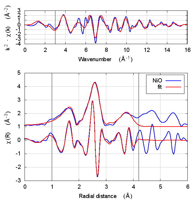 |
3.5 Discussion
NiO was chosen as the second example because it constitutes the smallest added complexity compared to copper. NiO is a rock salt structure, so it is highly ordered and the local configuration around the Ni atom is very well known. With an oxygen ligand, there should be some charge transfer.
With the exception of the E0 parameter, all of the parameters are constant well within their error bars. The statistical parameters are unchanged from model to model.
This is the first example of dependence of the E0 parameter on theoretical model. The ultimate value of Feff’s threshold energy depends on the model. The starting condition is not the same in Feff6 as in Feff8 without self-consistency. This is seen by the 3.3 eV shift in fitted E0 value. Furthermore, the threshold changes as charge is transferred and self-consistency is reached. This results in a -6 eV shift relative to Feff6.
My standard explanation of the E0 fitting parameter when I am teaching EXAFS is that it is the parameter that lines up the zero of wavenumber in the data with the zero of wavenumber in the theory. As such, it is hard to say that one of these E0 results is “better” than the others.
One might hope that improvements in theory would lead to a fitted E0 parameter of 0 when the edge is chosen at the inflection point of the rising edge of the XAS data. While that might be true, we’re not there yet with Feff8. See the conclusion for more discussion.
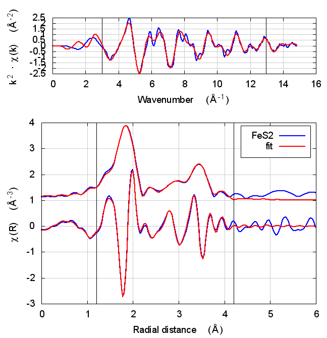
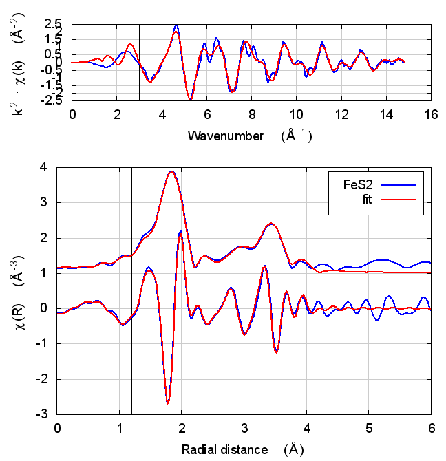
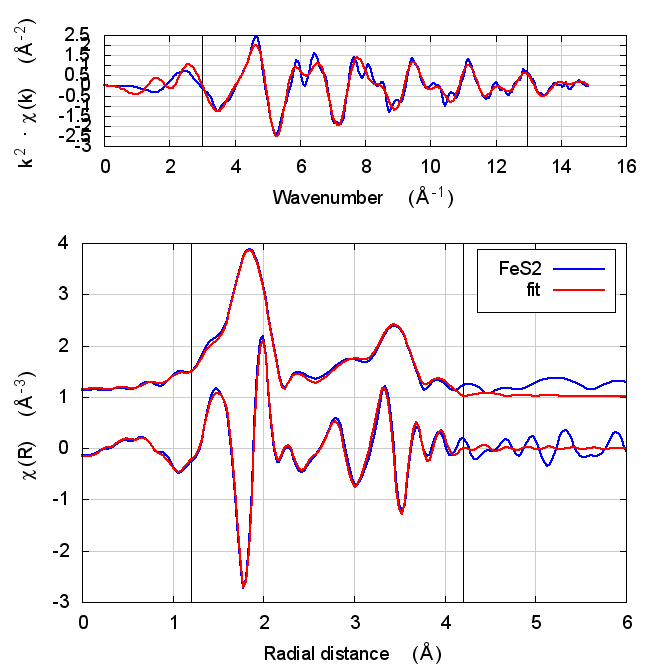
4 FeS2
This is one of my standard teaching examples. It’s good for teaching as it is fairly simple – it’s cubic – but it has a bit of structure and two kinds of scatterers. The data are taken from Matt's online collection of references.
The model includes a S0² parameter (amp), an energy shift (enot),
and a volumetric lattice expansion coefficient (alpha). The first and
second shell S scatterers each get a σ² parameter (ss and ss2). The
third shell of S atoms only contains 2 scatterers. In practice, floating
its σ² parameter independently does not yield a statistical improvement
to the fit, so the ss2 parameter is used for the third shell σ².
Finally a σ² parameter is floated for the Fe shell.
The fitting model includes a variety of multiple scattering paths, including a triangle between the first shell S and the fourth shell Fe, and four paths that bounce around among first shell S atoms.
amp and alpha are unitless. enot is eV. ss, ss2, and ssfe
are Ų.
4.1 Best fit values
| model | alpha | amp | enot | ss | ss2 | ssfe |
|---|---|---|---|---|---|---|
| feff6 | 0.00092(126) | 0.69(2) | 2.77(42) | 0.00296(41) | 0.00366(106) | 0.00484(50) |
| noSCF | 0.00183(171) | 0.65(3) | 7.01(57) | 0.00294(57) | 0.00386(151) | 0.00471(68) |
| withSCF(3) | 0.00219(191) | 0.68(3) | -2.01(63) | 0.00311(63) | 0.00422(172) | 0.00495(77) |
| withSCF(3.6) | 0.00212(188) | 0.68(3) | -2.15(62) | 0.00311(62) | 0.00423(170) | 0.00495(76) |
| withSCF(4) | 0.00212(191) | 0.68(3) | -2.17(63) | 0.00311(63) | 0.00423(172) | 0.00494(77) |
| withSCF(5.3) | 0.00216(194) | 0.68(4) | -1.92(64) | 0.00310(64) | 0.00421(175) | 0.00493(78) |
| withSCF(5.5) | 0.00216(194) | 0.68(4) | -1.88(64) | 0.00310(64) | 0.00421(175) | 0.00493(78) |
4.2 Statistics
| model | χ² | reduced χ² | R-factor |
|---|---|---|---|
| feff6 | 2052.3016 | 146.4407 | 0.0064 |
| noSCF | 3783.2180 | 269.9491 | 0.0119 |
| withSCF(3) | 4639.2799 | 331.0329 | 0.0146 |
| withSCF(3.6) | 4502.7226 | 321.2889 | 0.0141 |
| withSCF(4) | 4634.9046 | 330.7207 | 0.0145 |
| withSCF(5.3) | 4778.2793 | 340.9511 | 0.0150 |
| withSCF(5.5) | 4798.0987 | 342.3653 | 0.0151 |
4.3 Charge transfer and threshold energy
| ip | R=3 | R=3.6 | R=4 | R=5.3 | R=5.5 |
|---|---|---|---|---|---|
| 0 | -0.332 | -0.346 | -0.359 | -0.378 | -0.376 |
| 1 | -0.325 | -0.346 | -0.380 | -0.396 | -0.397 |
| 2 | 0.164 | 0.175 | 0.192 | 0.200 | 0.201 |
| μ | -9.464 | -9.555 | -9.671 | -9.488 | -9.465 |
Starting value for μ in feff8 = -0.796
Value for μ in feff6 = -4.308
4.4 Fits
| feff6 | no SCF | SCF, R=3 | SCF, R=3.6 | SCF, R=4 | SCF, R=5.3 | SCF, R=5.5 |
|---|---|---|---|---|---|---|
 |
 |
 |
 |
 |
 |
 |
4.5 Discussion
This is just slightly more complex than NiO. It is diatomic, but with a slightly less orderly structure than NiO. Again, all parameters except for E0 are consistent within uncertainty, although the α parameter does show some correlation with E0. All other parameters are essentially unchanged.
The E0 parameter, with self-consistency, is equally far from 0 as for Feff6, although with a sign change.
There are a small handful of small MS paths with half-path-lengths within the fitting range but which are not included in this fit. This may account for the increase in reduced χ² and R-factor between Feff6 and Feff8.
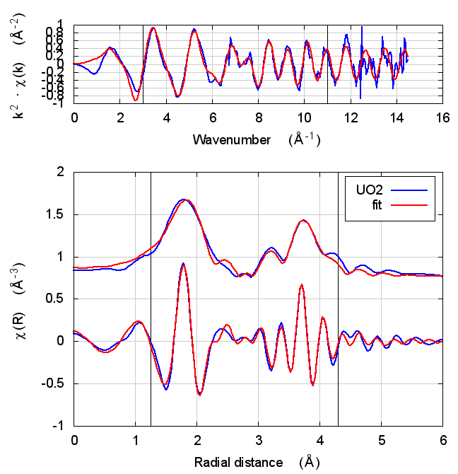
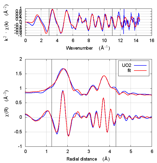
5 UO2
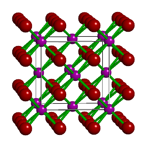
Figure 1: Uraninite
The data are the UO2 shown in Shelly’s paper on /Reduction of Uranium(VI) by Mixed Iron(II)/Iron(III) Hydroxide (Green Rust): Formation of UO2 Nanoparticles/: DOI: 10.1021/es0208409
This is an interesting test as it is an f-electron system.
The fitting model follows rather closely to what is described in that
paper, particularly the content of Table 2, although I allow S0² to
float (amp). Along with an energy shift (enot), a ΔR and σ² for the
first shell O (dro and sso), a ΔR and σ² for the second shell U
(dru and ssu), and a ΔR and σ² for the third shell O (dro2 and
sso2), there is a parameter for the number of U scatterers (nu).
The model includes the same 6 paths given in Table 2 of Shelly’s paper.
amp is unitless. enot is eV. dro, dru, and dro2 are Å. sso,
ssu, and sso2 are Å2.
5.1 Best fit values
| model | amp | dro | dro2 | dru | enot | nu | sso | sso2 | ssu |
|---|---|---|---|---|---|---|---|---|---|
| feff6 | 0.87(11) | -0.022(14) | -0.055(24) | 0.005(11) | 4.87(136) | 11.43(481) | 0.00939(213) | 0.01060(440) | 0.00488(247) |
| noSCF | 0.84(11) | -0.023(15) | -0.024(32) | 0.001(12) | 8.15(146) | 9.27(416) | 0.00872(221) | 0.01061(618) | 0.00382(273) |
| withSCF(3) | 0.84(10) | -0.026(13) | -0.013(28) | -0.002(11) | 1.63(129) | 9.21(376) | 0.00894(209) | 0.00976(511) | 0.00393(250) |
| withSCF(4) | 0.84(10) | -0.026(13) | -0.013(29) | -0.003(11) | 2.08(130) | 9.16(373) | 0.00892(209) | 0.00972(513) | 0.00389(250) |
| withSCF(5) | 0.84(10) | -0.026(13) | -0.012(28) | -0.003(11) | 1.72(129) | 9.18(373) | 0.00893(208) | 0.00969(508) | 0.00391(249) |
| withSCF(5.5) | 0.84(10) | -0.026(13) | -0.012(28) | -0.003(11) | 1.62(129) | 9.17(372) | 0.00894(208) | 0.00970(509) | 0.00391(249) |
| withSCF(6) | 0.84(10) | -0.026(13) | -0.012(29) | -0.003(11) | 1.71(129) | 9.16(372) | 0.00893(208) | 0.00971(510) | 0.00390(249) |
5.2 Statistics
| model | χ² | reduced χ² | R-factor |
|---|---|---|---|
| feff6 | 166.2736 | 22.0712 | 0.0160 |
| noSCF | 188.4320 | 25.0125 | 0.0181 |
| withSCF(3) | 169.5918 | 22.5116 | 0.0163 |
| withSCF(4) | 169.9560 | 22.5600 | 0.0163 |
| withSCF(5) | 169.1192 | 22.4489 | 0.0163 |
| withSCF(5.5) | 169.1306 | 22.4504 | 0.0163 |
| withSCF(6) | 169.2412 | 22.4651 | 0.0163 |
5.3 Charge transfer and threshold energy
| ip | R=3 | R=4 | R=5 | R=5.5 | R=6 |
|---|---|---|---|---|---|
| 0 | 1.122 | 1.146 | 1.180 | 1.189 | 1.191 |
| 1 | 0.715 | 0.726 | 0.740 | 0.745 | 0.741 |
| 2 | -0.363 | -0.369 | -0.376 | -0.379 | -0.377 |
| μ | -8.541 | -8.114 | -8.522 | -8.624 | -8.542 |
Starting value for μ in feff8 = -0.640
Value for μ in feff6 = -6.058
5.4 Fits
| feff6 | no SCF | SCF, R=3 | SCF, R=4 | SCF, R=5 | SCF, R=5.5 | SCF, R=6 |
|---|---|---|---|---|---|---|
 |
 |
 |
 |
 |
 |
 |
5.5 Discussion
The first thing to notice about UO2 is that the statistical parameters of the fit are completely unchanged between theory models.
This E0 parameter is the first one that behaves in the expected way – with self-consistency and charge transfer, the fitted E0 ends up closer to 0. Perhaps this is a hint that self-consistency is important for f-electron systems.
All of the other fitting parameters are unchanged within their
uncertainties. One parameter merits a bit more discussion. In the paper
cited above, the fitted value of nu, i.e. the partial occupancy of the
U atom in the second scattering shell, is used to say something about
the size of the uraninite nanoparticles generated by the reduction
process. While the fitted value of nu does not change outside of its
very large uncertainty, it does change substantively. This would likely
effect the interpretation of the fitting results in the context of the
reduction process.
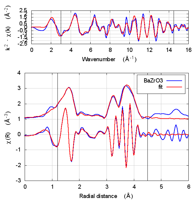
6 BaZrO3
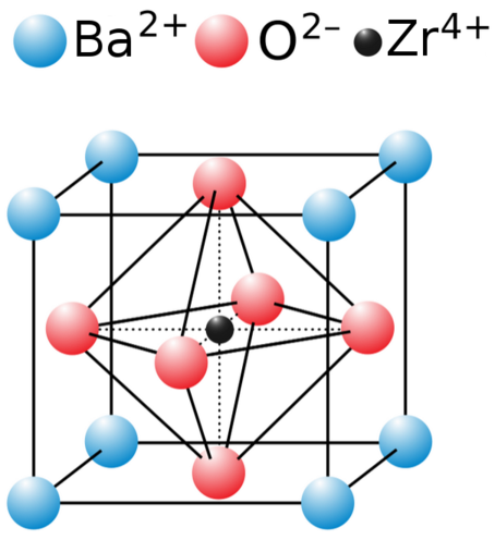
Figure 2: The perovskite structure.
In a short paper on the Zr edge of BaZrO3, DOI: 10.1016/0921-4526(94)00654-E, Haskel et al. proposed that shortcomings of feff’s potential model could be accommodated by floating an energy shift parameter for each scatterer species. The concept is that doing so approximates the effect of errors in the scattering phase shifts.
The data are the same as in that paper, although the fitting model is
slightly different. Rather than floating ΔR parameters for each shell, I
used a volumetric expansion coefficient (alpha). Along with S0²
(amp), there are energy shifts for each scatterer (enot, ezr, and
eba) and σ² parameters for each scatterer (sso, sszr, and ssba.
The fourth shell O is included in the fit. It gets a σ² (sso2) but
uses the energy shift for the O scatterer.
BaZrO3 is a true perovskite. Zr sites in the octahedral B site. A variety of co-linear multiple scattering paths at the distance of the third shell Zr scatterer are included in the fit. The energy shifts are parameterized as described in the paper.
amp and alpha are unitless. enot, ezr, and eba are eV. sso,
sszr, ssba, and sso2 are Ų.
6.1 Best fit values
| model | alpha | amp | eba | enot | ezr | ssba | sso | sso2 | sszr |
|---|---|---|---|---|---|---|---|---|---|
| feff6 | -0.00032(85) | 1.22(7) | -9.906(567) | -8.55(57) | -5.597(1717) | 0.00561(37) | 0.00403(70) | 0.00908(253) | 0.00413(33) |
| noSCF | 0.00044(86) | 1.07(6) | -3.901(589) | -2.32(58) | 0.946(1886) | 0.00530(38) | 0.00361(70) | 0.00791(242) | 0.00369(34) |
| withSCF(3) | -0.00007(72) | 1.13(5) | -10.768(469) | -10.52(47) | -6.682(1580) | 0.00561(32) | 0.00382(58) | 0.00855(208) | 0.00362(28) |
| withSCF(4) | -0.00007(74) | 1.13(5) | -11.026(482) | -10.60(48) | -6.794(1618) | 0.00559(33) | 0.00380(59) | 0.00850(213) | 0.00362(28) |
| withSCF(5) | -0.00007(73) | 1.13(5) | -11.094(479) | -10.81(48) | -7.057(1604) | 0.00561(33) | 0.00381(59) | 0.00850(211) | 0.00363(28) |
| withSCF(5.5) | -0.00007(73) | 1.13(5) | -10.950(477) | -10.77(48) | -7.050(1594) | 0.00562(33) | 0.00382(59) | 0.00850(210) | 0.00364(28) |
| withSCF(6) | -0.00005(73) | 1.13(5) | -10.705(474) | -10.49(48) | -6.726(1590) | 0.00562(33) | 0.00382(59) | 0.00851(208) | 0.00364(28) |
6.2 Statistics
| model | χ² | reduced χ² | R-factor |
|---|---|---|---|
| feff6 | 8979.2479 | 555.6561 | 0.0108 |
| noSCF | 9536.0604 | 590.1130 | 0.0114 |
| withSCF(3) | 6579.0004 | 407.1234 | 0.0079 |
| withSCF(4) | 6898.9084 | 426.9200 | 0.0083 |
| withSCF(5) | 6837.1517 | 423.0984 | 0.0082 |
| withSCF(5.5) | 6790.5892 | 420.2170 | 0.0081 |
| withSCF(6) | 6690.0972 | 413.9983 | 0.0080 |
6.3 Charge transfer and threshold energy
| ip | R=3 | R=4 | R=5 | R=5.5 | R=6 |
|---|---|---|---|---|---|
| 0 | 0.250 | 0.313 | 0.279 | 0.244 | 0.218 |
| 1 | 0.607 | 0.546 | 0.607 | 0.653 | 0.628 |
| 2 | 0.535 | 0.561 | 0.528 | 0.495 | 0.494 |
| 3 | -0.381 | -0.370 | -0.379 | -0.383 | -0.375 |
| μ | -7.698 | -7.958 | -8.036 | -7.902 | -7.600 |
Starting value for μ in feff8 = -1.336
Value for μ in feff6 = -6.654
6.4 Fits
| feff6 | no SCF | SCF, R=3 | SCF, R=4 | SCF, R=5 | SCF, R=5.5 | SCF, R=6 |
|---|---|---|---|---|---|---|
 |
 |
 |
 |
 |
 |
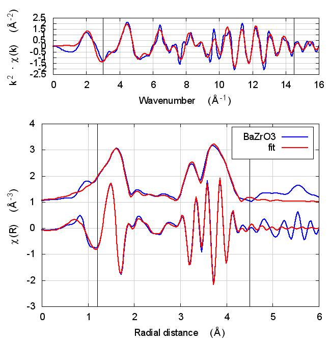 |
6.5 Discussion
In the paper cited above, the authors speculate that inaccuracies in Feff’s potential model can be accommodated by allowing separate E0 parameters to float for each kind of scatterer. In the paper, the claim is that the ΔR parameters used to model low temperature BaZrO3 data correctly follow the trends seen in high temperature XRD data on the same material.
I didn’t quite use the same fitting model as in that paper. Instead of a variety of ΔR parameters, I used a single isotropic expansion coefficient, α. With just one data set, the fit using many ΔR parameters was not stable.
The hope, in this case, is that self-consistency and charge transfer would make all the E0 parameters close to 0 and remove the need for multiple E0 parameters in the fit. Neither of those hopes were realized. The E0 parameters in the self-consistent fits were not much different from the results of the Feff6 fit and none of them ended up near 0.
Other fitting parameters were, as in other materials, consistent within uncertainties. In this case, the reduced χ² and R-factor were a bit lower with self-consistency with relative reductions on the same scale as the increases in FeS2 and NiO.
7 Bromoadamantane
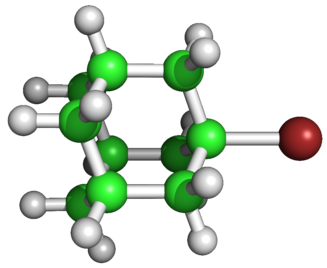
Figure 3: 1-bromoadamantane
The data are 1-bromoadamantane. Bromoadamantane is a cycloalkane, meaning that it is a hydrocarbon with rings of carbon atoms. It is also a diamondoid, meaning that it is a strong, stiff, 3D network of covalent bonds. 1-bromoadamantane has one hydrogen atom replaced by a bromine atom.
The material was supplied by my colleague Alessandra Leri of Manhattan Marymount College in the form of a white powder. This powder was spread onto Kapton tape which was folded to make a sample with an edge step of about 1.7. The data were measured by Bruce at NSLS beamline X23A2.
This is an interesting test case because it is a molecule (thus the entire molecule can be included in the self-consistency calculation) and because there is measurable scattering from the neighboring hydrogen atoms. While the σ² of the hydrogen scatterers is not well-determined, the fit is statistically significantly worse when the hydrogen scatterers are excluded.
The fit includes the nearest neighbor C, the next three C atoms, and the neighboring 6 hydrogen atoms. The DS triangle paths involving the first and second neighbor C atoms are also included.
ΔR parameters are floated for the nearest neighbor carbon, the second neighbor carbon, and the hydrogen scatterers. The adamantane anion is taken to be quite rigid compared to the Br-C bond, so the second neighbor σ² parameter is constrained to scale geometrically (i.e.\ by the square of the ratio of the fitted distances) from the σ² for the nearest neighbor.
7.1 Best fit values
| model | amp | delr | drc | drh | enot | ss | ssh |
|---|---|---|---|---|---|---|---|
| feff6 | 1.35(18) | 0.018(11) | -0.013(17) | 0.031(22) | 5.66(1.39) | 0.00522(144) | 0.00294(327) |
| noSCF | 1.11(13) | 0.014(12) | -0.021(19) | 0.076(24) | 10.97(1.37) | 0.00405(137) | 0.00145(326) |
| withSCF(8) | 1.20(12) | 0.014(10) | -0.017(15) | 0.070(24) | 0.57(1.20) | 0.00431(119) | 0.00363(370) |
7.2 Statistics
| model | χ² | reduced χ² | R-factor |
|---|---|---|---|
| feff6 | 3928 | 938 | 0.010 |
| noSCF | 4656 | 1112 | 0.012 |
| withSCF(8) | 3516 | 839 | 0.009 |
7.3 Charge transfer and threshold energy
| ip | R=8 |
|---|---|
| 0 | 0.468 |
| 1 | 0.024 |
| 2 | -0.047 |
| μ | -6.087 |
Starting value for μ in feff8 = 4.480
Value for μ in feff6 = -2.673
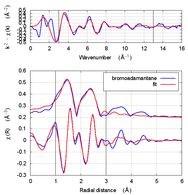
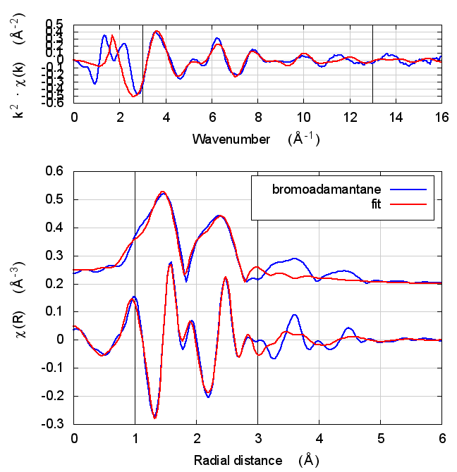
7.4 Fits
| feff6 | no SCF | SCF, R=8 |
|---|---|---|
 |
 |
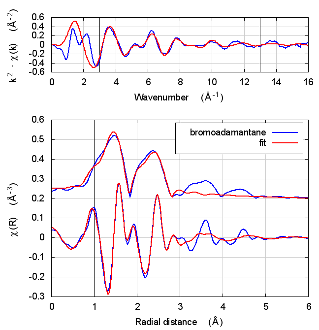 |
7.5 Discussion
In June 2015, the following quote appeared on the Ifeffit mailing list:
There are some demonstrated cases where Feff8 is slightly
better than Feff6 at modeling EXAFS. The most notable cases
are when H is in the input file -- Feff6 is terrible at this.
Bromoadamantane is a case where scattering from H atoms can be seen in the EXAFS data. The statistical parameters are all much smaller when the H SS path is included in the fit compared to fits which exclude that scattering path. This is true even though the σ² value for the H SS path is ill-determined – its uncertainty is such that σ² for H is not positive-definite. This is likely because the small mass of the H atom makes its partial pair distribution function highly non-Gaussian. The approximation of a simple σ² to model this distribution is not all that good. Despite the ill-defined σ², the ΔR is well defined.
The parameters of the first shell C scatterer are quite well defined and consistent across theory models. S0² varies to the limit of its uncertainty and ΔR for the H atom varies outside its uncertainty. The statistical parameters for the fits with self-consistency and Feff6 are basically indistinguishable.
So, is Feff6 “terrible” at handling H scatterers? The answer may be “yes” and may be “no”, but these data on bromoadamantane don’t suggest that it is any worse than Feff8.
8 Uranyl hydrate
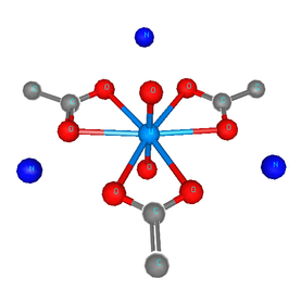
Figure 4: The uranyl motif from sodium uranyl triacetate.
The data are the hydrated uranyl hydrate shown in Shelly’s paper on X-ray absorption fine structure determination of pH-dependent U-bacterial cell wall interactions, DOI: 10.1016/S0016-7037(02)00947-X
This is an interesting test case because it involves very short ~1.78Å oxygenyl bonds in an f-electron system.
The AFOLP card was used to run feff6. The FOLP card with a value
of 0.9 for each potential was used to get feff8.5 to run to
completion.
Following the lead of that paper, feff was run on the crystal sodium uranyl triacetate. The relevant bit of the structure is shown in the figure. For the fitting model, scattering paths related to the axial and equatorial O atoms (red balls) are used in the fit. Other paths are unused. The parameterization given in Tables 2 and 5 is used in this fit.
There is an S0² (amp) and an energy shift (enot). The axial and
equatorial oxygen atoms each get a ΔR (deloax and deloeq) and a σ²
(sigoax and sigoeq).
amp is unitless. enot is eV. deloax and deloeq are Å. sigoax
and sigoeq are Ų.
8.1 Best fit values
| model | amp | deloax | deloeq | enot | sigoax | sigoeq |
|---|---|---|---|---|---|---|
| feff6 | 0.93(4) | 0.03504(396) | -0.04278(770) | 10.63(60) | -0.00007(53) | 0.00726(94) |
| noSCF | 1.04(6) | 0.03684(523) | -0.05319(975) | 11.32(78) | 0.00032(72) | 0.00699(118) |
| withSCF(2.5) | 1.08(6) | 0.04165(548) | -0.04475(972) | 3.45(81) | 0.00074(73) | 0.00692(115) |
| withSCF(2.9) | 1.08(6) | 0.04172(547) | -0.04485(971) | 3.50(81) | 0.00074(73) | 0.00691(115) |
| withSCF(4.0) | 1.08(6) | 0.04144(545) | -0.04455(969) | 3.59(81) | 0.00075(73) | 0.00694(115) |
| withSCF(5.2) | 1.08(6) | 0.04154(545) | -0.04473(967) | 3.66(81) | 0.00074(72) | 0.00693(114) |
| withSCF(6.8) | 1.08(6) | 0.04163(545) | -0.04478(968) | 3.63(81) | 0.00074(72) | 0.00693(114) |
8.2 Statistics
| model | χ² | reduced χ² | R-factor |
|---|---|---|---|
| feff6 | 37.6972 | 6.0758 | 0.0027 |
| noSCF | 69.0909 | 11.1356 | 0.0049 |
| withSCF(2.5) | 71.0295 | 11.4480 | 0.0050 |
| withSCF(2.9) | 70.8922 | 11.4259 | 0.0050 |
| withSCF(4.0) | 70.4038 | 11.3472 | 0.0050 |
| withSCF(5.2) | 70.2351 | 11.3200 | 0.0050 |
| withSCF(6.8) | 70.3644 | 11.3408 | 0.0050 |
8.3 Charge transfer and threshold energy
| ip | R=2.5 | R=2.9 | R=4.0 | R=5.2 | R=6.8 |
|---|---|---|---|---|---|
| 0 | 1.496 | 1.487 | 1.464 | 1.474 | 1.467 |
| 1 | -0.590 | -0.582 | -0.620 | -0.639 | -0.633 |
| 2 | -1.585 | -1.600 | -1.527 | -1.542 | -1.546 |
| 3 | -0.325 | -0.329 | -0.292 | -0.303 | -0.310 |
| 4 | -0.160 | -0.154 | -0.173 | -0.168 | -0.168 |
| 5 | 0.628 | 0.625 | 0.626 | 0.630 | 0.632 |
| μ | -2.810 | -2.751 | -2.629 | -2.569 | -2.587 |
Starting value for μ in feff8 = 6.030
Value for μ in feff6 = -1.961
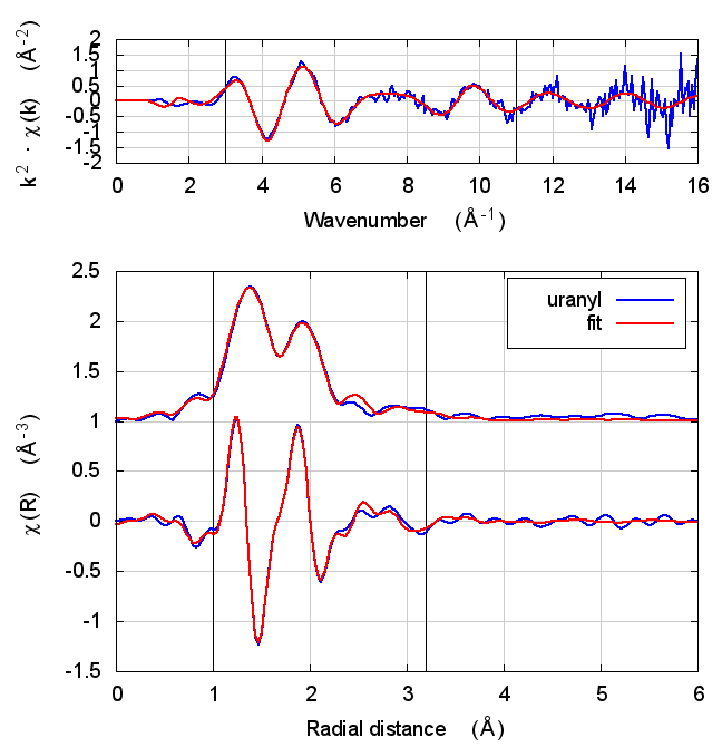
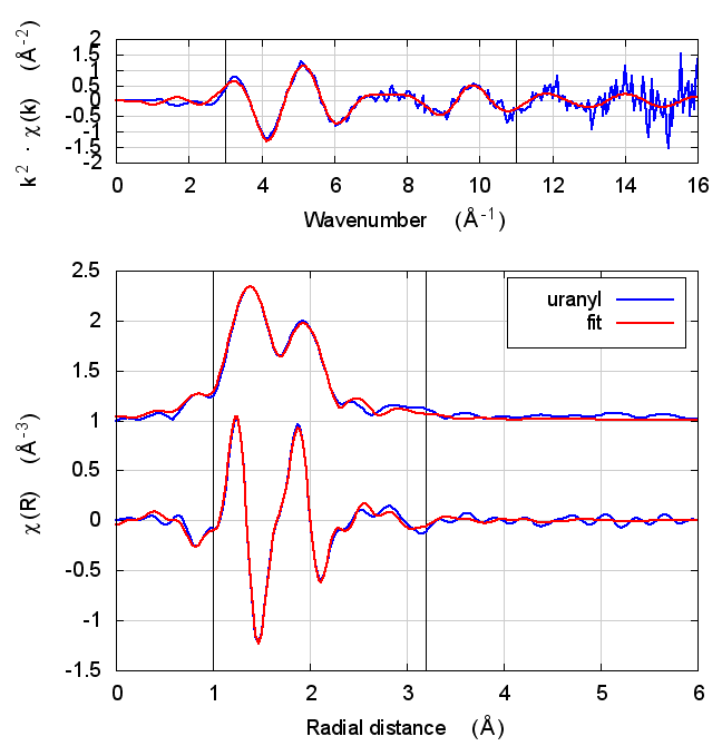
8.4 Fits
| feff6 | no SCF | SCF, R=2.5 | SCF, R=2.9 | SCF, R=4 | SCF, R=5.2 | SCF, R=6.8 |
|---|---|---|---|---|---|---|
 |
 |
 |
 |
 |
 |
 |
8.5 Discussion
The most interesting part of this fit is the extremely short, double bonded, axial oxygen scattering path. With such an extremely rigid bond, σ² is hard to determine. Even the most sensible result in the table above gives an answer that is barely positive-definite.
Beyond that parameter, the story here is, by now, familiar. Most fitting parameters are consistent over the theory models. This is one of the cases where the statistical parameters are slightly better for Feff6 than for any of the Feff8 fits.
Like with UO2, the E0 values of the self-consistent fits are what one hopes to find. They are much closer to zero when the edge energy of the data is chosen at the inflection point of the rising edge. Is this a trend suggesting that self-consistency is important for setting the energy scale of f-electron systems?
Also like the UO2 example, the S0² value is a bit different using Feff6 and Feff8, which could have an impact on the interpretation of the data. It is, however, correlated with the axial σ² result.
9 Conclusion
Sometimes (FeS2, uranyl) the statistical parameters suggest the best fit was found using Feff6. Sometimes (BaZrO3) Feff8 with self-consistency gave the smaller reduced χ² and R-factor. And sometimes (UO2) it made no difference.
Excepting E0 parameters, the fits presented here yielded equivalent values for fitting parameters using Feff6 and Feff8 with self-consistency. Only in the case of f-electron systems – UO2 and uranyl – were the fitting results for E0 parameters more sensible with Feff8 and self-consistency.
In most cases, the fit using Feff8 without self-consistency resulted in the largest statistical parameters.
Artemis has used Feff6 for years. Nothing presented here suggests that was a bad idea.
In the future, Artemis will likely use feff85exafs. It seems that the most sensible default behavior for Artemis would be to run feff85exafs using a very short self-consistency radius.
Is a reviewer justified in demanding that an author use a more recent version of Feff than Feff6? On the basis of what I have presented here, I think not.
9.1 Theoretical approximations and measurement uncertainty
The most valuable result of this effort – beyond the immediate question of the impact of self-consistent potentials on EXAFS analysis – is that these results provide a sense of what level of uncertainty is introduced to the application of Gaussian statistics to EXAFS analysis by uncertainties in the theory model used as the basis of the fitting.
This paper attempts to quantify many of the sources of uncertainty in an EXAFS measurement. The sort of comparison presented here offers hope of quantifying the contribution to the uncertainty budget of the measurement due to the approximations that enter into the theory.
9.2 Interpreting the E0 shift parameter
Way back in the early 1990s, in the days of Feff3, the theory was already good enough to get calculated, relative peak positions very consistent with experimental data in the EXAFS region. That is, the phase part of the calculation was already highly reliable for large photoelectron kinetic energies in the very earliest days of XAS theory.
Consider this paper on a leading contender for the best theoretical approach to XANES and XES, the Bethe-Salpeter equation of motion of the electron-hole pair. This is an impressive and successful approach to core-shell theory, however the positions of peaks in the density of states near the edge, both above and below, are clearly lacking. Consider the MgO calculation in Fig. 5 of that paper. It’s a great result, but the peaks are demonstrably shifted relative to experiment.
In the context of finding the threshold energy and the zero of photoelectron wavenumber, a misplacement of peaks in the DOS will result in a misplacement of the threshold. From the Feff3 results, we know that an E0 shift is adequate to position the high kinetic energy peaks well with respect to the data. Given the shortcomings even of the current most advanced theory with respect to finding the absolute energy threshold, it is clear that a parameter for an overall E0 shift remains necessary to line up the EXAFS data with the EXAFS theory. While one must remain mindful that fitted E0 shifts can be too large, thus confounding the measurement of other parameters, EXAFS analysis continues to require E0 shift parameters.
9.3 A note on the set of standards
For anyone doing EXAFS analysis, a fairly common moment is the one when a fit is not going well, the parameters don’t make sense, the fitted function doesn’t look like the data, and the person doing the analysis is deeply confused.
In that moment, it is extremely tempting to blame the theory. In fact, it is super fun to blame Feff. Don’t stop there! Blame John Rehr personally for your analysis woes. Fun and satisfying!
The truth is, that moment of confusion usually happens with a real research project and typically with a material for which the experimenter has rather little prior knowledge about the actual structure of the sample. While it is tempting to attribute a poor fit to an inadequacy of the theory, it is vastly more likely that the problem is a shortcoming of the fitting model.
In this exercise, I chose a set of materials for which I have excellent prior knowledge about the local configuration around the absorber. With a good structural model, any shortcomings of the fit would then more likely be attributable to shortcomings of the theory.
This exercise, along with my long experience, tell me that when you, dear reader, find yourself cursing Feff and/or John, you should indulge that only long enough to get it out of your system. Then you should think deeply about your sample and how you represent its structure in the fit. It is much more likely that your sample is something other than what you expect and that the solution to your problem is to prepare a better sample or to dream up a more representative fitting model.