10. Fitting EXAFS data
Here is a complete fitting example. In this example, data on a copper foil are fit using a model considering isotropic expansion and a correlated Debye model.
Everything up to line 44 should be familiar to you if you have read all the previous parts of this programming guide. An ATHENA project file is imported at line 5. A record from that project file is imported into a Data obejct at line 8 and various parameters of the Data object are set at lines 9-15.
A FEFF calculation is made at lines 17-19. Note the use of
chained method calls at line 19. This is possible because the
potph method returns the calling object. (So does pathfinder,
for that matter, although its return value is thrown away here.) The
path list is dereferenced for convenience at line 20.
Various guess and set parameters are defined at lines 23-28 and stored in an array. The parameters will be used to set up a simple fitting model consisting of an amplitude term, an E0 shift, an isotropic expnasion model for ΔR for each path, and a correlated Debye model for the σ2 for each path.
At lines 33-42, various Path objects are defined using the ScatteringPath objects from the FEFF calculation. The path parameters are assigned math expressions using the appropriate GDS parameters.
1 2 3 4 5 6 7 8 9 10 11 12 13 14 15 16 17 18 19 20 21 22 23 24 25 26 27 28 29 30 31 32 33 34 35 36 37 38 39 40 41 42 43 44 45 46 47 48 49 50 51 52 53 54 55 56 57 58 59 60 61 | #!/usr/bin/perl
use Demeter qw(:ui=screen);
## import an Athena project file with copper metal in it
my $prj = Demeter::Data::Prj->new(file='cu_data.prj');
## make a Data object and set the FT and fit parameters
my $data = $prj->record(1);
$data ->set(name => 'My copper data',
fft_kmin => 3, fft_kmax => 14,
fit_k1 => 1, fit_k3 => 1,
bft_rmin => 1.6, bft_rmax => 4.3,
fit_do_bkg => 0,
);
## run a Feff calculation on copper metal
my $feff = Demeter::Feff -> new(file => "cu_metal.inp");
$feff -> set(workspace => "cu_workspace/", screen => 0,);
$feff -> potph -> pathfinder;
my @list_of_paths = $feff-> list_of_paths;
## make GDS objects for an isotropic expansion, correlated Debye model fit to copper
my @gds = (Demeter::GDS -> new(gds => 'guess', name => 'alpha', mathexp => 0),
Demeter::GDS -> new(gds => 'guess', name => 'amp', mathexp => 1),
Demeter::GDS -> new(gds => 'guess', name => 'enot', mathexp => 0),
Demeter::GDS -> new(gds => 'guess', name => 'theta', mathexp => 500),
Demeter::GDS -> new(gds => 'set', name => 'temp', mathexp => 300),
Demeter::GDS -> new(gds => 'set', name => 'sigmm', mathexp => 0.00052),
);
## make Path objects for the first 5 paths in copper (3 shell fit)
my @paths = ();
foreach my $i (0 .. 4) {
$paths[$i] = Demeter::Path -> new();
$paths[$i]->set(data => $data,
sp => $list_of_paths[$i];
s02 => 'amp',
e0 => 'enot',
delr => 'alpha*reff',
sigma2 => 'debye(temp, theta) + sigmm',
);
};
## make a Fit object
my $fit = Demeter::Fit -> new(gds => \@gds,
data => [$data],
paths => \@paths
);
## do the fit
$fit -> fit;
## set up some plotting parameters
$data->po->set(plot_data => 1, plot_fit => 1,
plot_bkg => 0, plot_res => 0,
plot_win => 1, plot_run => 1,
kweight => 2,
r_pl => 'r',
);
$data->plot('r');
$data->pause;
|
As I said, everything up to this point has been covered already. The fitting magic happens at lines 45-48. A Fit object is defined as a collection of GDS, Data, and Path objects. Those three attributes of the Fit object each takes an anonymous array (as at line 46) or references to named arrays (as at lines 45 and 47). That's it! That's how you make a fit.
Although the first 42 lines of code do not constitute a substantial savings of effort compared to a writing FEFFIT input file or an IFEFFIT script in terms of the amount of typing that you have to do. That changes substantially once the fit is defined. When the fit is requested at line 52, DEMETER does a lot of work disentangle the contents of the arrays containing the GDS, Data, and Path objects. As discussed in an upcoming section extensive checks are run to confirm that all aspects of the fitting model make sense and that there are no obvious errors in the fitting model (e.g. guess parameters that are defined but not used).
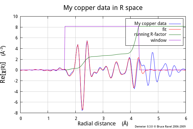
Fig. 10.1 Lines 54-58 in the script above defined how the plot at line 60 will appear. Various flags of the Plot object are set such that the data and fit are plotted alonmg with a window showing the fitting range and the running R-factor, which is a way of visualizing how the misfit is distributed over the fitting range. A k-weight of 2 is used to make the Fourier transform before the plot.
In the next section, we'll see how to do multiple data set fitting and how to incorporate more than one FEFF calculation in a fit. In later sections we will explore other features of the Fit object, including its extensive sanity checking, all the interesting things that can be done with the Fit object after a fit finishes, and a discussion of DEMETER's happiness parameter.
Contents
DEMETER is copyright © 2009-2016 Bruce Ravel – This document is copyright © 2016 Bruce Ravel
This document is licensed under The Creative Commons Attribution-ShareAlike License.
If DEMETER and this document are useful to you, please consider supporting The Creative Commons.