Setting up an EXAFS fit

In this section, the examples will reinforce the idea that the Fit object is simply a collection of Data, Path, and GDS objects. We have already seen some of this. To make a fit, a number of GDS object are created and the gds attribute of the Fit object is set to an anonymous array containing those GDS objects. Similarly, the paths attribute is set to an anonymous array containing all the Path objects to be used in the fit. This idea of a Fit object containing a collection of other objects extends to its use for more advanced fitting concepts. A Fit object for a multiple data set fit has its data attribute set to an anonymous list of Data objects. This is shown in the first example below. A Fit object involving multiple FEFF calculations is made by creating some number of Path objects from each FEFF calculation, then collecting all those Path objects into the paths attribute of the Fit object. This is shown in the second example below.

---

 

Multiple data set fitting

The following script expands upon the example in the previous section by expanding the isotropic expansion and correlated Debye fitting model to a simultaneous refinement of two data sets. In this example, two copper foils measurements were made at 10 K and 150 K. Both are imported from an ATHENA project file and a Fit object is established using both data sets.

#!/usr/bin/perl
use Demeter qw(:ui=screen);

## import an Athena project file with copper metal in it
my $prj = Demeter::Data::Prj->new(file='cu_data.prj');

## make a Data object and set the FT and fit parameters
my @data = $prj->records(1, 2);
$data[0] -> name('10 K copper data');
$data[1] -> name('150 K copper data');
my @common = (fft_kmin   => 3,        fft_kmax   => 14,
              fit_k1     => 1,        fit_k3     => 1,
              bft_rmin   => 1.6,      bft_rmax   => 4.3,
              fit_do_bkg => 0,
             );
$_ -> set(@common) foreach @data;

## run a Feff calculation on copper metal
my $feff = Demeter::Feff -> new(file => "cu_metal.inp");
$feff -> set(workspace => "cu_workspace/", screen => 0,);
$feff -> potph -> pathfinder;
my @list_of_paths = $feff-> list_of_paths;

## make GDS objects for an isotropic expansion, correlated Debye model fit to copper
my @gds =  (Demeter::GDS -> new(gds => 'guess', name => 'alpha10',  mathexp => 0),
            Demeter::GDS -> new(gds => 'guess', name => 'alpha150', mathexp => 0),
            Demeter::GDS -> new(gds => 'guess', name => 'amp',      mathexp => 1),
            Demeter::GDS -> new(gds => 'guess', name => 'enot',     mathexp => 0),
            Demeter::GDS -> new(gds => 'guess', name => 'theta',    mathexp => 500),
            Demeter::GDS -> new(gds => 'set',   name => 'sigmm',    mathexp => 0.00052),
           );

## make Path objects for the first 5 paths in copper (3 shell fit)
my @paths = ();
foreach my $i (0 .. 4) {
  ## paths for data at 10K
  $paths[$i] = Demeter::Path -> new();
  $paths[$i]->set(data     => $data[0],
                  sp       => $list_of_paths[$i];
                  s02      => 'amp',
                  e0       => 'enot',
                  delr     => 'alpha10*reff',
                  sigma2   => 'debye(10, theta) + sigmm',
                 );

  ## paths for data at 150K
  my $j = $i+5;
  $paths[$j] = $paths[$i] -> Clone;
  $paths[$j] -> set(data     => $data[1],
                    delr     => 'alpha150*reff',
                    sigma2   => 'debye(150, theta) + sigmm',
                   );
};

## make a Fit object
my $fit = Demeter::Fit -> new(gds   => \@gds,
                              data  => \@data,
                              paths => \@paths
                             );

## do the fit
$fit -> fit;

## set up some plotting parameters
$data[0] -> po -> set(plot_data => 1,   plot_fit  => 1,
                      plot_bkg  => 0,   plot_res  => 0,
                      plot_win  => 0,   plot_run  => 0,
                      kweight   => 2,
                     );
$data[0] -> y_offset(6);
$_ -> plot('rmr') foreach @data;
$data[0] -> pause;

This script bears a strong resemblance to the one in the previous section. There are a couple of small differences. At lines 8-16, two records are imported from the ATHENA project file. They both have parameters set appropriately. One fewer GDS object at lines 19-25 is defined compared to the previous script. This is because the temperature parameter of IFEFFIT's debye function is explicitly set to the correct value at lines 43 and 51.

The major difference of this multiple data set fitting model is at line 57. Both Data objects are supplied to the Fit object. This is the fundamental difference between a single and multiple data set fit -- the number of items in the Fit object's data attribute. Very cool!

Another major difference is shown at lines 47-52. In those lines a set of Path objects is set up and associated with the second Data object. At lines 37-44, Path objects are set up for the 10 K data in identical manner to the script in the previous section. At line 48, each Path object is cloned, returning a new Path object with all the same attributes. These copies are added to the @paths list, with care taken at line 47 to do the counting correctly. In lines 49-52, only those parameters that need to be changed to be appropriate for the 150 K data set are set to their new values. At line 49, the cloned paths are associated with the 150 K Data object. At lines 50 and 51, the temperature dependent path parameters are set appropriately.

Note that the sp atrtibute is not changed for the cloned paths. This is central to DEMETER's efficient use of FEFF. The same ScatteringPath object is used for the Path object associated with the 10 K Data object and for the Path object associated with the 150 K Data object. This is conceptually equivalent to using the same feffNNNN.dat file in two different path paragraphs in a FEFFIT input file.

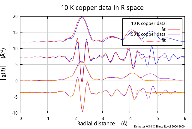
Another impoirtant thing demonstrated by this example is how a fairly elaborate polot can be generated with a small number of lines of code. The plot to the right is what gets made by lines 65-71. Lines 65-69 set some parameters of the Plot object. Line 70 sets a vertical offset for the plot of the 10 K data. At line 71 Rmr plots are made for each Data object. That's a lot of plot for two lines of code!

---

 

Using multiple Feff calculations