4.4. Plot object

The Plot object is used to control the details of how plots are made and displayed by DEMETER programs. It is useful to consider how ATHENA works in order to understand the relationship of the Plot object to the rest of DEMETER. In ATHENA, the plot controls are separate from the controls for the parameters of any individual data set. For example, the range over which data are plotted in energy or R-space is, in some, sense, a global parameter not associated with a particular data set. The Plot object serves this role. The details of the plot in DEMETER are global. To plot a plottable object (Data, Path, or any of the Path-like objects), DEMETER consults the Plot object for those details.

To make the Plot object readily accessible at all times in your program, the po method is a method of the base class and is inherited by all DEMETER objects. Thus, given any object, you can “find” the Plot object like so:

$the_plot_object = $any_object -> po;

Any method of the plot object is easily called by chaining with the po method. For example to start a new plot (as opposed to overplotting), you do this

$any_object -> po -> start_plot;

The start_plot method reinitializes the Plot object to begin a new plot. Along with clearing the plotting display, this restarts the trace colors and resets the plot title.

4.4.1. Plotting in energy

4.4.1.1. Data, background, pre-edge, & post-edge

my @eplot = (e_mu      => 1,     e_bkg     => 1,
             e_norm    => 0,     e_der     => 0,
             e_pre     => 1,     e_post    => 1,
             e_i0      => 0,     e_signal  => 0,
             e_markers => 1,
             emin      => -200,  emax      => 2000,
             space     => 'E',
            );
$data -> po -> set(@eplot);
$data -> po -> start_plot;
$data -> plot;

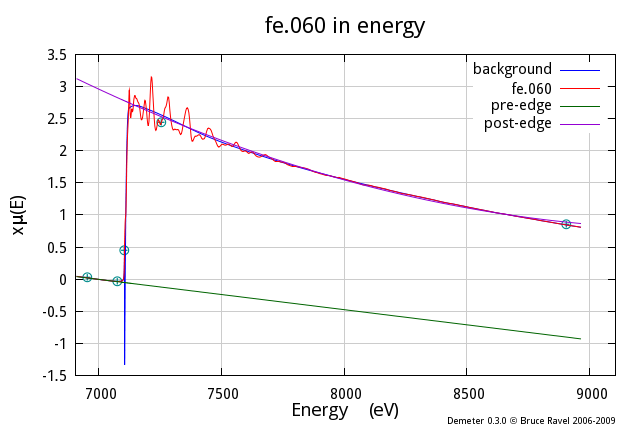
Fig. 4.1 This example demonstrates the common and useful plot showing the data along with the background function and the regressed polynomials used to normalize the data. Note that the Plot object has a number of boolean attributes which turn features of the energy plot on and off. Also note that the range of the plot is set by the values of the emin and emax attributes of the Plot object.

Also note that, as was discussed in the chapter on the Data object, there is no need to explicitly perform the data normalization or background removal. DEMETER knows what needs to be done to bring the data up to date for plotting and will perform all necessary chores before actually generating the plot. This allows you to focus on what you need to accomplish.

One final point about this example. I have created the @eplot array to hold the attributes of the Plot object. I then pass that array as the argument of the set method of the Plot object. Those attributes could be listed as explicit arguments of the set method. As always in perl, there's more than one way to do it.

4.4.1.2. Normalized data & background

my @eplot = (e_mu      => 1,     e_bkg     => 1,
             e_norm    => 1,     e_der     => 0,
             e_pre     => 0,     e_post    => 0,
             e_i0      => 0,     e_signal  => 0,
             e_markers => 1,
             emin      => -200,  emax      => 2000,
             space     => 'E',
            );
$data -> po -> set(@eplot);
$data -> bkg_flatten(0);
$data -> po -> start_plot;
$data -> plot;

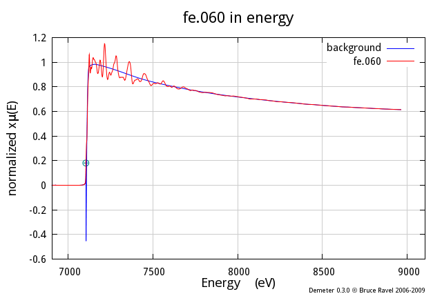
Fig. 4.2 This example shows how to plot data and background function after normalization.

4.4.1.3. Flattened data & background

my @eplot = (e_mu      => 1,     e_bkg     => 1,
             e_norm    => 1,     e_der     => 0,
             e_pre     => 0,     e_post    => 0,
             e_i0      => 0,     e_signal  => 0,
             e_markers => 1,
             emin      => -200,  emax      => 2000,
             space     => 'E',
            );
$data -> po -> set(@eplot);
$data -> bkg_flatten(1);
$data -> po -> start_plot;
$data -> plot;

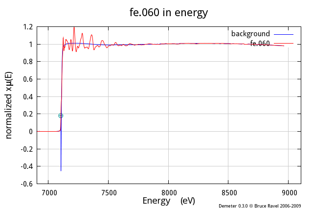
Fig. 4.3 This example shows how to plot the flattened data and background function, that is, the normalized data with the difference in slope and quadrature between the pre- and post-edge lines subtracted out after the edge.

Note that the switch for turning flattening on and off is an attribute of the Data object not the Plot object. This allows the option of overplotting one data set that is normalized with another that is flattened.

4.4.1.4. Derivative of mu

my @eplot = (e_mu      => 1,     e_bkg     => 0,
             e_norm    => 0,     e_der     => 1,
             e_pre     => 0,     e_post    => 0,
             e_i0      => 0,     e_signal  => 0,
             e_markers => 0,
             emin      => -20,   emax      => 120,
             space     => 'E',
            );
$data -> po -> start_plot;
$data -> set(name=>'derivative') -> plot;
$data -> po -> e_norm(1);
$data -> set(name=>'norm. deriv.') -> plot;

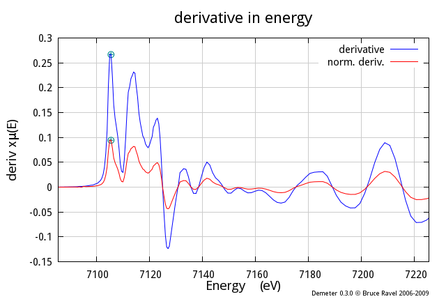
Fig. 4.4 This shows how things get overplotted, in this case the derivative of μ(E) and the derivative of normalized μ(E).

This example shows two interesting features we haven't yet seen. The overplotting happens simply by calling the plot mthod a second time without calling start_plot. In this way, any number of things can be overplotted.

Also note the use of chained method calls to set the Data object's name attribute appropriately before plotting. The name method always returns the object that called it, which allows for this sort of chaining magic to happen. There is no advantage to chained method calls – you could rename the Data object and then plot it in the subsequent line. The cahined calls are a bit more concise.

4.4.1.5. Data, I0 channel, & signal channel

my @eplot = (e_mu      => 1,     e_bkg     => 0,
             e_norm    => 0,     e_der     => 0,
             e_pre     => 0,     e_post    => 0,
             e_i0      => 1,     e_signal  => 1,
             e_markers => 0,
             emin      => -20,   emax      => 120,
             space     => 'E',
            );
$data -> po -> start_plot;
$data -> plot;

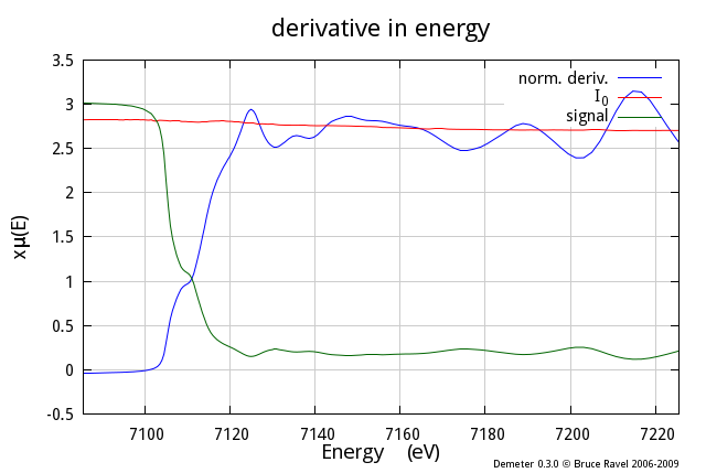
Fig. 4.5 DEMETER saves arrays containing I₀ and the signal channel, which can then be plotted along with the data. DEMETER takes care to scale these arrays so that they plot nicely with the data.

4.4.1.6. Data at two different edges with E0 subtracted

my @common = (bkg_rbkg    => 1.5,
              bkg_spl1    => 0,    bkg_spl2    => 18,
              bkg_nor2    => 1800,
              bkg_flatten => 1,
             );
my @data = (Demeter::Data -> new(),
            Demeter::Data -> new(),
           );
foreach (@data) { $_ -> set(@common) };
$data[0] -> set(file => "$where/data/fe.060.xmu",
                name => 'Fe 60K', );
$data[1] -> set(file => "$where/data/cu010k.dat",
                name => 'Cu 10K', );

## decide how to plot the data
$plot -> set(e_mu    => 1,   e_bkg   => 0,
             e_norm  => 1,
             e_pre   => 0,   e_post  => 0,
             e_zero  => 1,
             emin    => -30, emax    => 150,
            );
$data[0] -> po -> start_plot;
foreach (@data) { $_ -> plot('E') };

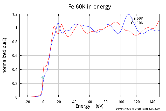
Fig. 4.6 DEMETER offers an easy way to plot μ(E) data with the E₀ value subtracted. This places the edge at 0 on the x-axis, allowing you to overplot data from different edges. When the e_zero attribute of the Plot object is set to 1, each Data object's bkg_eshift attribute is temporarily set so that the edge will show up at 0 in the plot.

4.4.2. Plotting in k

4.4.2.1. Plotting in k-space

$data -> po -> start_plot;
$data -> po -> kweight(2);
$data -> plot('k');

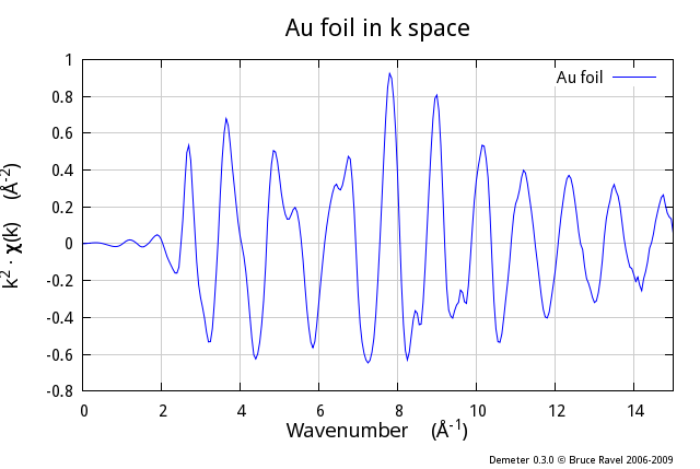
Fig. 4.7 Again, DEMETER will take care of the background removal when you request a plot in k-space. Note that the k-weight to use for plotting is an attribute of the Plot object.

4.4.2.2. Plotting in chi(k) in energy

$data -> po -> start_plot;
$data -> po -> set(kweight=>2, chie=>1);
$data -> plot('k');

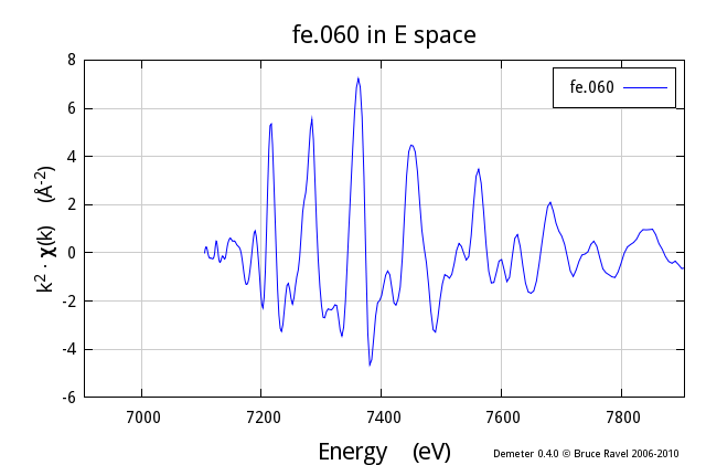
Fig. 4.8 Here the x-axis of the χ(k) plot has been converted to absolute energy.

4.4.2.3. k-space with all three k-weights

$data -> po -> start_plot;
$data -> plot('k123');

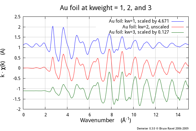
Fig. 4.9 DEMETER has several types of interesting, pre-defined plots. One of these, the “k123 plot”, will overplot the data three times, once each with k-weight values of 1, 2, and 3. The copy of the data with k-weight of two is plotted normally. The other two copies are scaled up or down to be about the same size as the k-weight of 2 copy. The data are analyzed and the scaling and offset constants are chosen to be appropriate to the data.

4.4.3. Plotting in R

4.4.3.1. Magnitude in R-space & R-space window

$data -> po -> set(kweight => 2, r_pl => 'm', space => 'r', );
$data -> po -> start_plot;
$data -> plot -> plot_window;

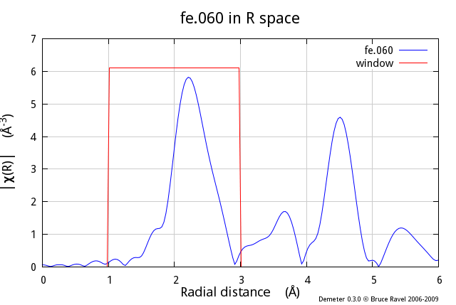
Fig. 4.10 This example shows a common kind of plot, χ(R) data with the back-Transform windowing function, which is also used by DEMETER as the fitting range when a fit is evaluated in R-space. The r_pl attribute of the Plot object is set to m, indicating that the magnitude of χ(R) should be plotted.

Note that the plot_window method was indicated in a chained method call. This is not required, but is possible because the plot method returns the calling object.

The plot_window method observes the value of the Plot object's space attribute. That is, if the plot s being made in k or q, the k-space window will be plotted. If the plot is being made in R, the R-space window will be plotted.

4.4.3.2. Data in R-space as envelope, real part, & imaginary part

$data -> po -> set(kweight => 2, r_pl => 'e', space => 'r');
$data -> po -> start_plot;
$data -> plot;

$data -> set(name=>'Real part');
$data -> po -> set(r_pl => 'r', );
$data -> plot;

$data -> set(name=>'Imaginary part');
$data -> po->set(r_pl => 'i', );
$data -> plot;

$data -> set(name=>'fe.060');  ## reset original name

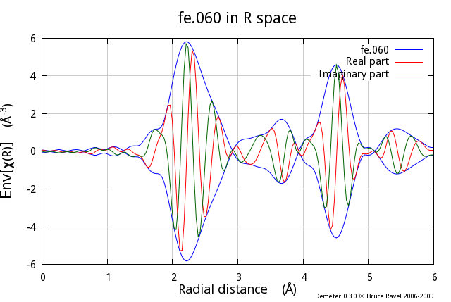
Fig. 4.11 Multiple parts of the complex χ(R) are overplotted by repeatedly plotting data in R-space without calling the start_plot method. The value of r_pl is set between each part of the plot. Note that the “envelope” is the magnitude plotted twice, multiplied by -1.

4.4.3.3. R-space with all three k-weights

$data -> po -> start_plot;
$data -> plot('r123');

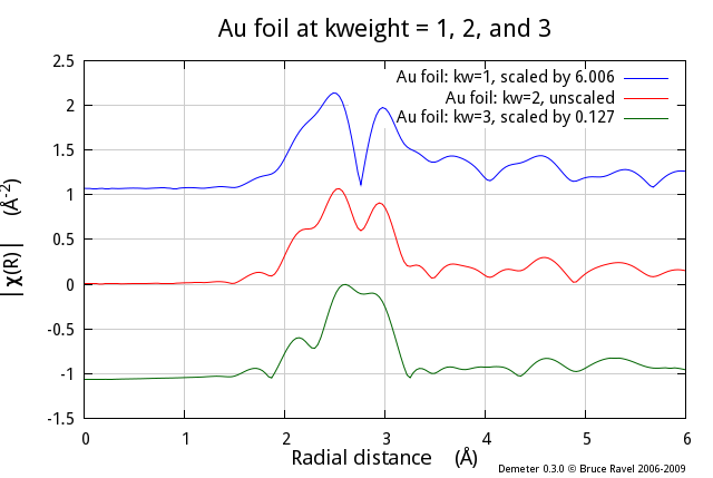
Fig. 4.12 The “R123 plot” is another pre-packaged specialty plot types. This one, is just like the “k123” plot in that three copies of the data are overplotted using each of the three k-weights with scaling and offset computed automatically. This “R123” plot was plotted as the magnitude of χ(R). The “R123” plot respects the value of the r_pl attribute of the Plot object.

4.4.3.4. Magnitude and real part in R space

$data -> po -> start_plot;
$data -> po -> kweight(2);
$data -> plot('rmr');

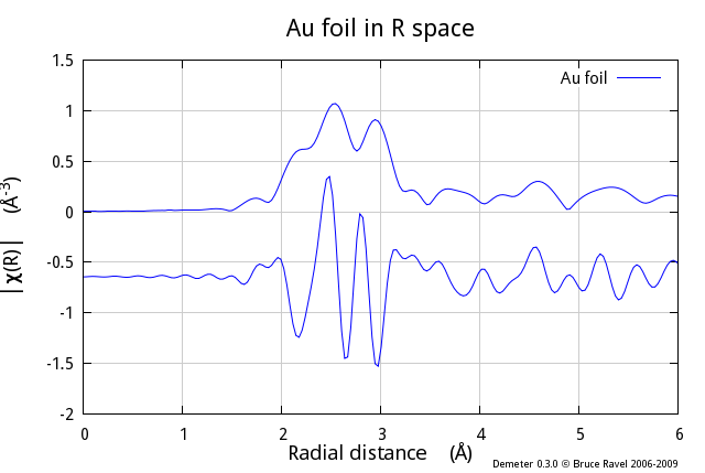
Fig. 4.13 The “Rmr plot” is the third of the pre-packaged specialty plot types. This one plots the magnitude and real part of χ(R) with an appropriate offset between them. This is the default plot type made after a fit finishes. In that case, the data and fit are overplotted as magnitude and real.

4.4.4. Plotting in q

4.4.4.1. Plotting in back-transform k-space

$data -> po -> set(kweight => 2, q_pl => 'r');
$data -> po -> start_plot;
$data -> plot('q');

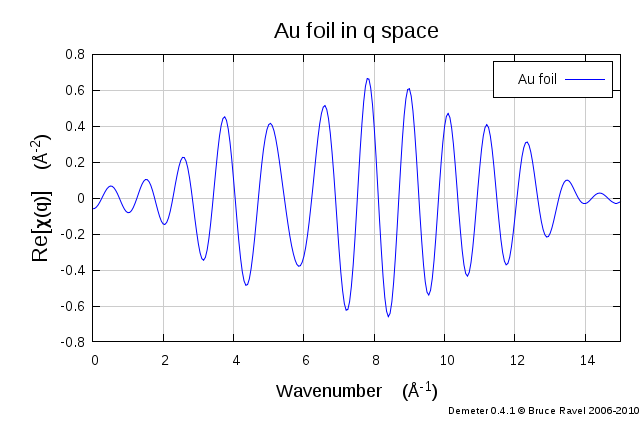
Fig. 4.14 Plotting the back-transformed χ(q) is specified by plotting in q. The part of the complex χ(q) is specified using the q_pl attribute of the Plot object.

4.4.4.2. k-space & the real part of back-transform k-space

$data -> po -> start_plot;
$data -> po -> kweight(2);
$data -> plot('kq');

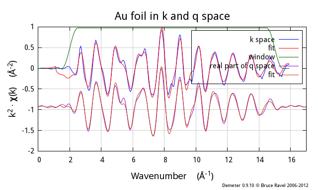
Fig. 4.15 Another specialty plot type in DEMETER, the “kq plot”. This overplots χ(k) with the real part of χ(q).

---

DEMETER is copyright © 2009-2016 Bruce Ravel – This document is copyright © 2016 Bruce Ravel

This document is licensed under The Creative Commons Attribution-ShareAlike License.

If DEMETER and this document are useful to you, please consider supporting The Creative Commons.