Linear combination fitting

Interpreting data as a mixture of standards

ATHENA has a capability of fitting a linear combination of standard spectra to an unknown spectra. These fits can be done using normalized μ(E), derivative of μ(E), or χ(k) spectra. One use of this sort of analysis might be to interpret the kinetics of series of spectra measured during a reduction reaction. By fitting each intermediate spectrum as a linear combination of the end members, one can deduce the rate of the reaction. Another possible use would be to determine the species and quantities of standards in a heterogeneous sample.

A worked example of linear combination fitting is shown later in this manual.

To access this feature, choose “Linear combination fit” from the main menu. The normal parameter view will be replaced by the tool in the following figure for performing the linear combination fit.

---

 

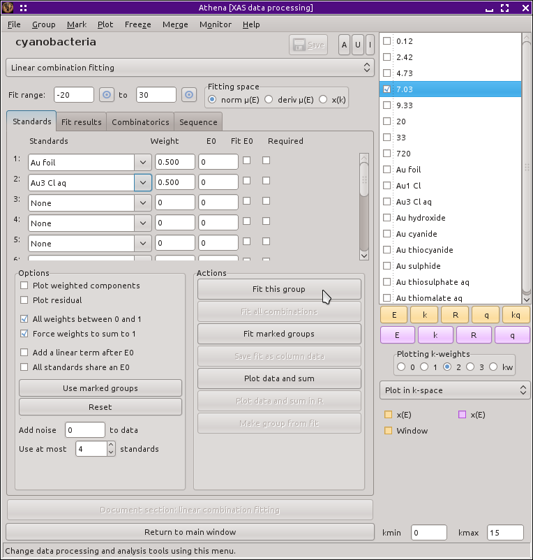
Fitting a single data group

The linear combination tool presents a table of menus. Each of these menus can be used to select a spectrum from among the data groups currently in the Data groups list. The basic idea of this tool is that you will choose two or more standard spectra and fit a linear combination of them to the current (i.e. the one highlighted in pale red in the Data groups list) group. The fitting is done using the normalized μ(E) spectra. If the standards or the unknown are to be flattened, then the flattened spectrum will be used. (See the section on background removal for details about flattened spectra.)

You should have already done some data processing on the standards and on the unknowns. Specifically, you should align your data and set appropriate normalization parameters for each spectrum before starting to use the linear combination fitting tool. Failing to adequately prepare your data for these fits will certainly result in questionable fits.

To do the fit, weighting parameters are defined for each standards spectrum except for the last one in the list. The weight for the last spectrum is one minus the sum of the other weights, thus constraining the standards to be 100 percent of the unknown. Thus, if you used three standards, the first two would have weights x and y and the third would have weight 1-x-y. x and y would then be varied to best fit the data. Each standard spectrum is interpolated onto the energy grid of the unknown when the fit is performed as normalized or derivative μ(E). The fit is performed over the data range indicated by the text boxes near the top of the window. There are pluck buttons which can be used to set the fitting range by clicking on a plot of the data.

Fitting normalized μ(E), derivative μ(E), or χ(k) is chosen using the radio buttons just above the table of standards. When fitting χ(k) spectra, you have the option of fitting a single spectrum to the data.

When fitting normalized or derivative μ(E) spectra, you have the option of floating an E₀ for each standard independently. This is intended to fix up any inconsistencies in the energy alignment of the various spectra (although it is much better to do a good job of aligning your data before doing your linear combination fitting). These E₀ variables can be introduced by clicking on the checkbuttons in the table of standard spectra.

You can introduce a linear offset to the fit to normalized μ(E) spectra. This is simple a line added to the sum of spectra in the fit. It introduces two parameters to the fit, a slope and an intercept. The line is multiplied by a step function centered at the E₀ of the unknown. Thus the linear offset is introduced only after the edge of the unknown. The purpose of this offset is to accommodate any variations in how the normalization is performed on the various spectra. To turn on the linear offset in the fit just click on the button labeled “Add a linear term after e0?”

For best results, you should do a good job of aligning and normalizing your spectra before starting linear combination analysis. When normalization and alignment are done correctly, you can expect your fitted weights to sum to 1 and variation of E₀ for the data or standards will be unnecessary.

---

 

Constraints and modifications to the fit

ATHENA's linear combination tool offers several constraints to the fitting parameters. The constraints are set and unset using the checkbuttons near the bottom of the tool.

Weights between 0 and 1

You can constrain the variable weights to be between 0 and 1 by clicking on the button labeled “Weights between 0 & 1.” In this case, each weight used is computed from the variable using this formula:

     guess  weight_varied = 0.5
     def    weight        = max(0, min(1, weight_varied))

The weight reported at the end of the fit, then, is the result of that formula. Note that the use of the min/max idiom means that uncertainties cannot be calculated for situations where the guess variable gets pinned to 0 or 1. That can happen in situations where one or more of the standards used in the fit is not appropriate to the data and is an indication that you should rethink the set of standards used in the fit. When this option is not selected, the guessed variable itself is used as the weight in the fit and is not prevented from being negative or larger than 1.

Force weights to sum to 1

You can loosen the constraint that the weights sum to 1 by deselecting the final checkbutton. This allows the final weight to float freely along with the rest rather than constrain it to equal 1 minus the sum of the rest, as described above. Loosening this constraint might yield fit results that are hard to interpret. If the constraint that weights must be between 0 and 1 is in place, then the weight of the last standard in the fit is computed by this formula:

   def  weight_final = max(0, 1 - (w1 + w2 + ... wn))

This forces the final weight to be positive, but may result in a fit that does have weights that, in fact, do not sum to one. Should that happen, it might be interpreted to mean that the normalization of the data or standards was not correct or that the choice of standards is not appropriate to the data.

Constrain all standards to use a single E0 shift

You can force all standards to use a single E₀ shift parameter in the fit. This is equivalent (albeit with a sign change) to fixing all the standards and using an E₀ shift on the unknown data.

Adding noise to the data

It is sometimes useful to check the robustness of the fit against noisy data. This is particularly true for a data set wherein some data are much noisier than others. To this end, ATHENA allows you to add pseudo-random noise to the data before performing the fit. This is done by generating an array of psuedo-random numbers and adding this array to the data. Given that normalized μ(E) is used in lCF fits, σ (the scale of the noise) has a simple interpretation -- it is a fraction of the edge step. A bit of trial and error might be necessary to find a suitable level of noise for your test. For fits to χ(k), note that the noise is added to the data before k-weighting. You can examine the level of noise relative to your data before fitting by using the “Plot data and sum” from the actions list.

Adding a linear term to the fit

A line with a variable slope and offset can be added to a fit. The line is only evaluated after the E₀ value of data being fit.

---

 

Fitting, statistics, reports

To perform the fit, click “Fit” from the actions list. After the fit finishes, the data and the linear combination will be plotted along with vertical bars indicating the range over which the fit was evaluated. The values of all the fitting parameters are written to the “Fit results” tab.

Interpretation of the statistical parameters in the linear combination fit is somewhat challenging. There are two reasons for this, both of which have to do with the fact that a non-linear, least-squares minimization is used in the analysis.

First, it is difficult (perhaps impossible) to quantify the number of independent measurements in the XANES spectrum. That number is certainly less than the number of data points measured. Nonetheless, when the chi-square is evaluated, the number of data points is used as the number of measurements.

Second, ATHENA has no way of evaluating a measurement uncertainty ε for the XANES measurement. A value of 1 is used for ε in the equation for chi-square.

These two issues, taken together, mean that chi-square and reduced chi-square tend to be very small numbers -- much smaller than 1. As a result, it is impossible to use reduced chi-square to evaluate the quality of a single fit. Relative changes in chi-square between fits are probably meaningful. However, given the two problems described above, chi-square does not have a very different meaning from the R-factor.

The R-factor reported in the text box is

    sum ( (data - fit)^2 )
   ------------------------
    sum (     data^2     )

where the sums are over the data points in the fitting region. The chi-square and reduced chi-square are those reported by IFEFFIT.

Interpretation of the statistical parameters requires you to be mindful of what you know about the system you are measuring. The statistical parameters alone are not sufficient to evaluate the fit results. The results of sample fractions must be meaningful in the context of any external knowledge you have about the system.

You can replot the data and the fit using the most recent values for the fitted parameters by clicking “Plot” in the actions list.

You can save the text from the fit results box to a file by clicking “Write a report” in the actions list. This writes a column data file with the fit results as the header information. The columns in the file are x-axis (either energy or k), the data, the best fit, the residual, and each of the weighted components.

You can make a data group out of the linear combination by clicking “Make fit group” in the actions list or out of the residual by clicking “Make difference group” in the actions list. This will allow you to plot and manipulate the fit or difference after leaving the linear combination tool. The data group containing the fit result will be treated as normal data that can have a background removed or be Fourier transformed. When you save a fit using the derivative spectra, the fit group will be saved as a normal μ(E) spectrum.

“Reset” in the actions list returns almost everything in the tool back to its original state.

If you need more than four standards, the number of standards as well as several other aspect of the linear combination fitting is configurable using the preferences tool.

---

 

Constraining linear combination fit parameters between groups

The various operational parameters described above can be constrained between data groups in the same manner as background removal and Fourier transform parameters on ATHENA's main page. Two items in the actions list are “Set params, all groups” and “Set params, marked groups”. These will export the current group's values for fitting range, noise, weights between 0 and 1, force weights to sum to 1, and use of linear term to other groups. This should probably be done before using the marked group fitting feature described in the next section.

---

 

Batch processing

One of the choices in the actions list is to “Fit marked groups”. All groups marked by having their purple buttons checked will be fit in the manner described above using the current selection of fitting standards and other fitting options. When the sequence of fits is finished, the “Write marked report” option will become enabled in the operation list. This will allow you to write a report in the form of a comma separated value file which summarizes the results of the sequence of fits. This report file can be read into any spreadsheet program.

Note that the report file will only reflect the fits done during the batch job. Any changes made to the fitting model will not be included in that report until a new batch job is performed.

Also note that the only way that the batch job is different from running the same sequence of fits by hand is that the report file can be generated. There is currently no way to generate a similar report from a sequence of fits not run using the batch processing option. However, you always have the option of saving individual fit reports as described above.

---

 

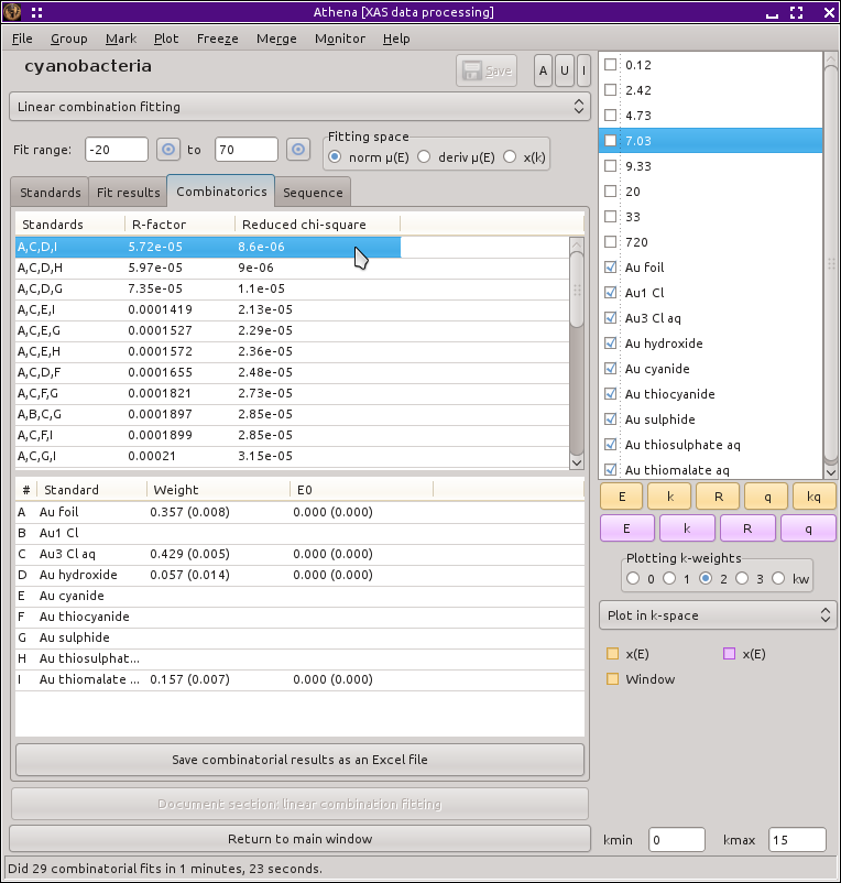
Combinatorial fitting using many standards

One of the uses of this sort of XANES fitting is to try to figure out what's actually in a sample. One approach to figuring this out is to measure all plausible standard compounds and try fitting a large number of different combinations of the standards to the data. ATHENA provides a tool for automating this. Here is how it works:

1. Load all of the standards that you want to consider into the table of standards in the linear combination tool. You may need to increase the maximum number of standards using the preferences tool to provide enough space in the table for all of the standards that you wish to consider.

2. You can limit the number of standards used in each fit with the incrementer widget just below the button marked “Use marked groups”. By default this number is 4, which says that the fits will consider all possible binary, ternary, and quaternary combinations of standards. Increase this number to consider higher orders of combinations of standards. Decrease it to limit the number of fits to perform. You can also indicate which standards are “required” by clicking the check button in the right-most column of the table of standards. This will limit the combinations of standards tested against to data to those that contain the required standards, thus greatly reducing the scope of the combinatorial problem.

3. Click “Fit all possible combinations” in the actions list and go get a cup of coffee. If the number of possible standards is large, this series of fits could take a while. For example, with 11 standards and considering up to the quaternary combinations, ATHENA will perform 550 fits. (Really! C(11, 2) + C(11, 3) + C(11, 4) = 550!)

Once this series of fits finishes, the tab labeled “Combinatorics” will become active and raise to the top. In this tab, you will see two tables. The top table concisely summarizes all the fits that were performed, in order of increasing R-factor. Initially, the first item in the list -- which has the lowest R-factor -- is selected (i.e. highlighted in pale red).

The second table contains each of the standards and its weight and E₀ from the fit selected in the upper table.

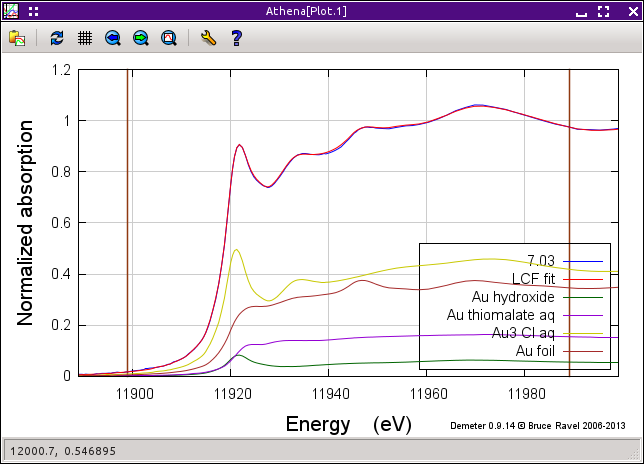
You can select a fit from the upper table by clicking on its line. When you do so, that fit becomes highlighted in pale red, its fitting results are inserted in the bottom table, its best fit function is plotted along with the data, and its results are inserted into the other two tabs. In this way, you can examine any fit from the series, as seen in the plot below.

Depending on the selection of standards, it is reasonable that two or more fits might have similar R-factors. You might interpret that to mean that those fits are statistically indistinguishable or you might be able to invoke some a priori knowledge to help choose between the similar fits. Other fits farther down in the list will be obviously worse both by statistical metric and by examination of their results.

Clicking the right mouse button on a fit in the upper table will post a context menu with options relevant to the selected fit. These options include saving the fit as a data group; writing a data file with columns for the data, fit, residual, and each weighted standard; saving the report from the “Fit results” tab to a file; and writing a comma-separated-value report for the entire combinatorial sequence which can be imported into a spreadsheet program.

Beneath the tables is a button labeled “Write CSV report for all fits.” Clicking this will prompt you for a file name and location, then write a comma-separated-value report of all fits.

A worked example of linear combination fitting is shown later in this manual.