Difference spectra

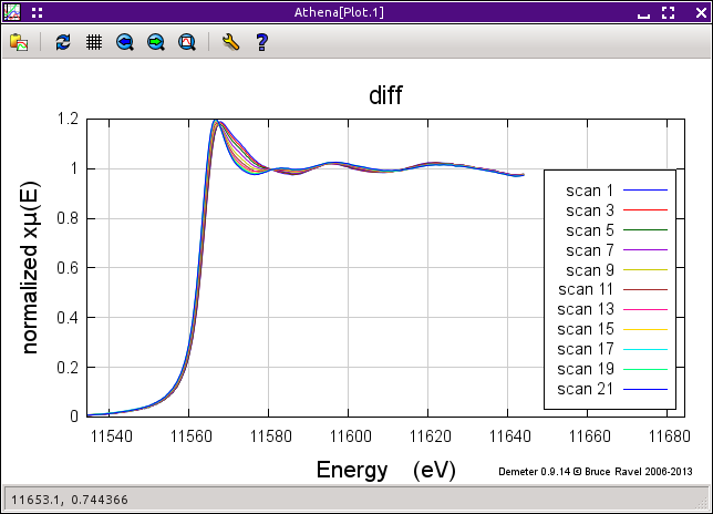
In many situations, the trends in a sequence measured data can be indicative of the of the physical process being measured. Shown in the figure below is a sequence of Pt L_III spectra measured on a hydrogenated Pt catalyst. In this sequence, the hydrogen is being desorbed, resulting in measurable changes in the spectra.

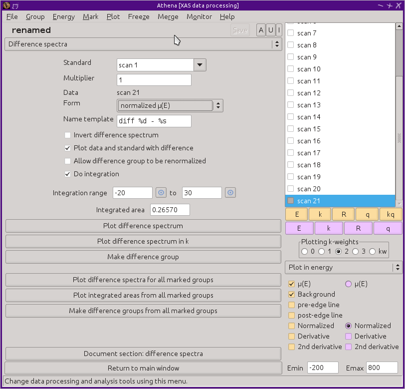
Selecting one of the difference spectra options from the main menu replaces the main window with the difference tool, as shown below. Difference spectra can be computed as μ(E), normalized μ(E), and derivative or second derivative of μ(E).

For difference spectra to be meaningful, it is essential that data processing be performed correctly for each data group. It is essential that you take great care with selecting parameters, calibrating, aligning, and all other processing chores.

As you click on each group in the group list, the difference spectrum is computed as the difference between the groups selected as the standard by menu control at the top of the window and the selected group from the group list. The difference spectrum will be plotted, optionally along with the data and standard used to make the subtraction. The form of the difference spectrum – μ(E), normalized μ(E), and derivative or second derivative of μ(E) – is selected from the menu labeled “Form”. The multiplier is a scaling factor that can be applied to the standard before subtraction.

If you have accidentally swapped the standard and data, click the “invert” button to change the order of the subtraction.

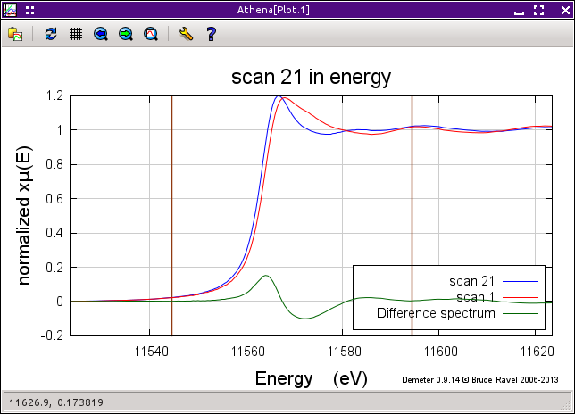
You can select two points, shown in the plot below by the brown markers, and integrate the area under that part of the spectrum.

The difference spectra saved to data groups. Those data groups are treated in every way like any other data group. By default, difference groups are marked as normalized groups – that is, a flag is set which skips the normalization algorithm. The “renomralize” button can be ticked to make the resulting group a normal μ(E) group. When the form of the difference is set to plain μ(E), that button will be ticked.

The name of the resulting data group will be set using the “Name template”, which includes a mini-language of tokens that will be substituted by specific values.

%d

Replaced by the name of the data group.

%s

Replaced by the name of the standard group.

%f

Replaced by the form of the difference spectrum

%m

Replaced by the multiplier value

%n

Replaced by the lower bound of the integration range

%x

Replaced by the upper bound of the integration range

%a

Replaced by the compted area over the integration range

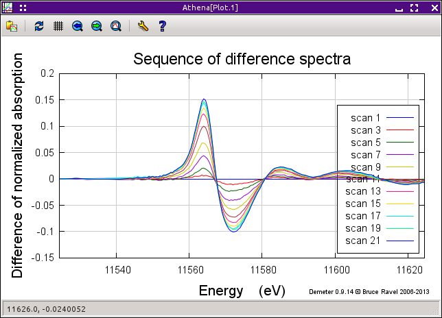
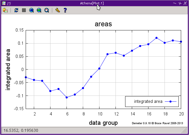
The integrated areas obtained by computing a sequence over all groups marked in the group list can be plotted by clicking the button labeled “Plot integrated areas for all marked groups.” The reult of this shown below.

---

 

Uses of difference spectra

Magnetic dichroism

This part of ATHENA is directly applicable to dichroism studies. The difference spectra is made in normalized μ(E) and the integration can be used to measure magnetic moments in magnetic materials.

Experimental corrections

Certain kinds of corrections for nonlinearities in the XAS measurement can be corrected by normalizing measured data by a blank scan – that is a measurement through the same energy range using the same instrumentation, but measured without the sample in the beam path. This sort of correction, as shown in C. T. Chantler, et al., J Synchrotron Radiat., 19, (2102) p. 851 (DOI: 10.1107/S0909049512039544), is equivalent to a difference spectrum measured in plain μ(E) between the data and balnk scan.