The Autobk Algorithm and the Rbkg Parameter

Understanding the most important background removal parameter

The frequency cutoff between the background and the data discussed in the previous section is determined by the «rbkg» parameter. This is the second parameter displayed in the background removal section of the main window.

When data are imported into ATHENA, «rbkg» is set to its default value, normally 1.

This example, like many of the examples in this Users' Guide, can be found at among the examples at my XAS-Education site.

Among these example files is one called fe.060, which contains a spectrum from an iron foil measured at 60 K. Import this by selecting Open file from the File menu or by pressing Control-o. Navigate to the location of your example files and select fe.060. The column selection dialog then appears. For now, just click OK.

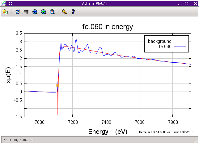
The data is imported and «rbkg» is set to its default value of 1. The data and the background function found using the default parameter values can be found by pressing the E button. This is shown here on the left.

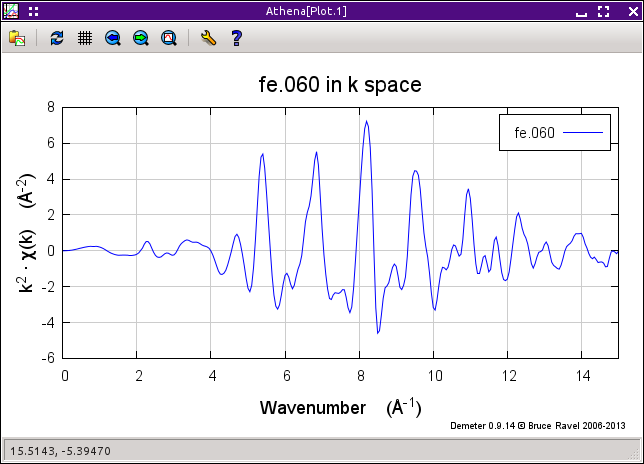
The background function is subtracted from the data and normalized, resulting in a χ(k) function. Press the k button to see χ(k), shown in the right panel above.

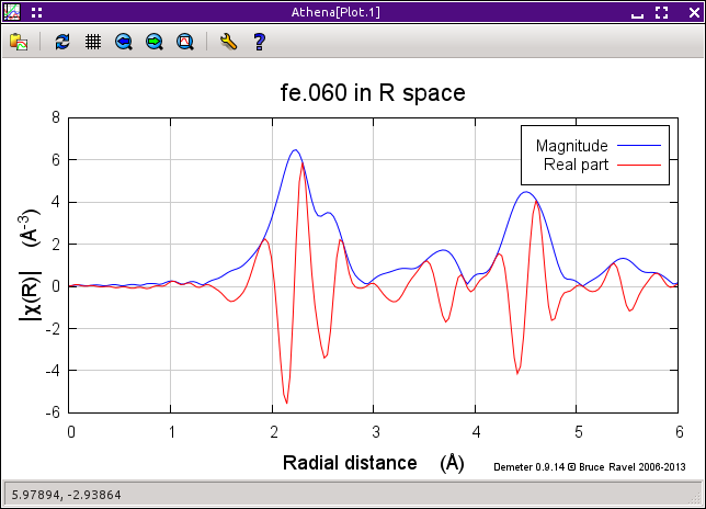
When you press the R button, the Fourier transform is plotted, as in the bottom panel above.

So «rbkg» is the value below which the AUTOBK algorithm removes Fourier components. As you can see, below 1 the χ(R) function is essentially 0, but above 1 the spectrum is non-zero.

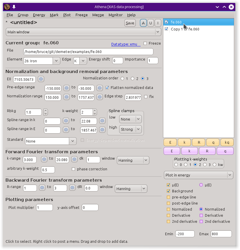
Now let's examine the effect of choosing different values for «rbkg». First, make a copy of the data so we can directly compare different values. Do that by selecting “Copy current group” from the Group menu or by pressing Shift-y. ATHENA now looks like this.

Click on the group Copy of fe.060 to display its parameters in the main window. Change «rbkg» to 0.2. Now we want to directly compare these two ways of removing the background. The way of plotting multiple items in the groups list involves the row of purple plotting buttons and the little check buttons next to the items in the group list. Click on the little check buttons next to fe.060 and Copy 1 of fe.060, as shown in the screenshot above. 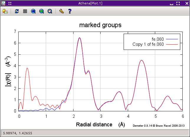Now plot these two items by clicking the R button. It should look something like this.

I suspect the blue spectrum is something like what you expect EXAFS data to look like, while the red one seems somehow worse. In fact, it is easy to understand why the red one looks the way it does. The «rbkg» parameter specifies the R value below which the data is removed from the μ(E) spectrum. That is exactly what has happened in the red spectrum -- below 0.2 the signal is very small and the first big peak is, in fact, above 0.2.

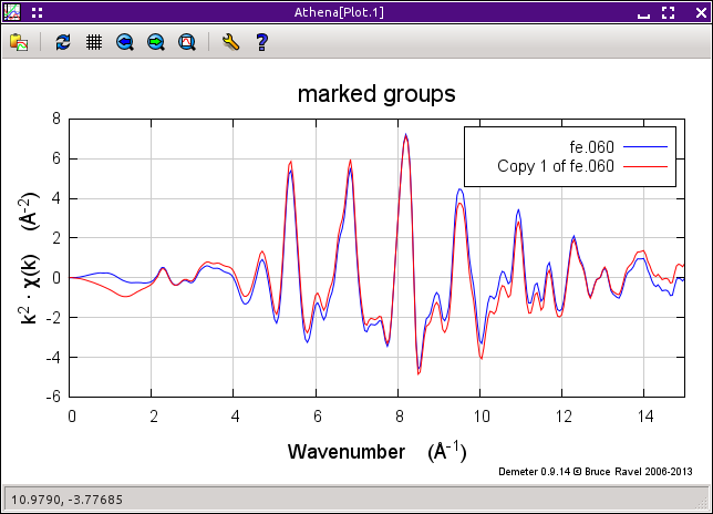
Those two, plotted as χ(k), are shown above on the right.

The blue spectrum oscillates around the zero axis, as one would expect. The red one has an obvious, long-wavelength oscillation. It is that oscillation that gives rise to the low-R peak in the χ(R) spectrum.

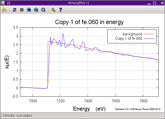
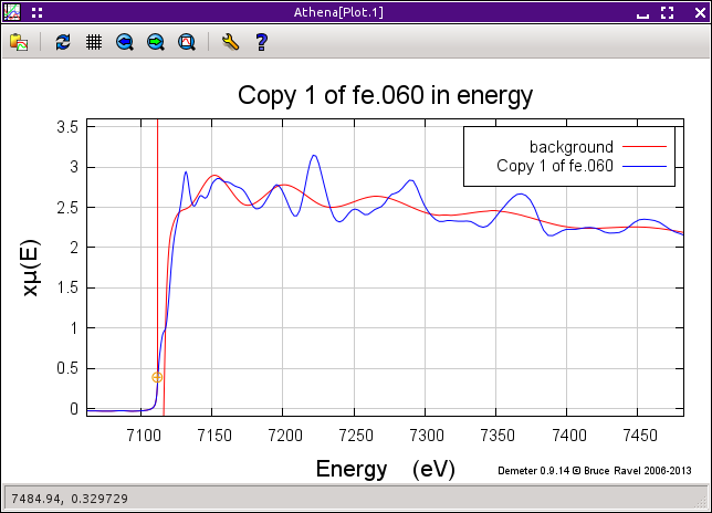
The background function, computed using 0.2 as the value of «rbkg» and plotted in energy, is shown above in the bottom panel.

Using an «rbkg» value of 0.2 yields a background function that is not able to follow the actual shape of the data.

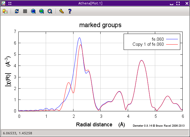
What happens if the value of «rbkg» is set to a very large value? The χ(R) data for the values 1 and 2.5 are shown here.

Using a very large value of «rbkg» results in significant change to the first peak in χ(R). We can see why by looking at the background function in energy . With such a large value of «rbkg», the background function has enough freedom to oscillate with frequencies that resemble the data. This results in a reduction of intensity under the first peak.

The spline used to compute the background function has a limited amount of freedom to oscillate. The number of spline knots is determined by the Nyquist criterion. This number is proportional to the extent of the data in k-space multiplied by «rbkg». These knots are spaced evenly in wavenumber. Thus the spline function can only have frequency components below «rbkg».

So where does that leave us? We want to make «rbkg» as big as possible so that the low-R peaks are as well suppressed as possible. On the other hand, too large of a value will result in damage to the data. The trick is to find a balance.

A good rule of thumb is that «rbkg» should be about half the distance to the nearest neighbor. But that is only a rule of thumb. Real data can be really difficult. Noisy data, data with strong white lines, data truncated by the appearance of another edge -- all of these require careful consideration. While «rbkg» is the primary background removal parameter, several others should be investigated to yield a good background removal. Several of these are the subjects of the following sections.