12.2. Linear combination analysis

12.2.1. Using XANES data and LCF to study system kinetics

This section outlines the linear combination fitting analysis of an experiment to study the kinetics of the reduction of aqueous Au³⁺ chloride to metallic gold. The experiment is described and these data are presented in

• Maggy F. Lengke, Bruce Ravel, Michael E. Fleet, Gregory Wanger, Robert A. Gordon, and Gordon Southam. Mechanisms of Gold Bioaccumulation by Filamentous Cyanobacteria from Gold(III)−Chloride Complex. Environmental Science & Technology, 40(20):6304–6309, 2006. doi:10.1021/es061040r.

The experiment probed the mechanism of bioaccumulation of gold by the interaction of a model cyanobacterium (Plectonema boryanum UTEX 485) with aqueous Au³⁺ chloride. This resembles a common subsurface environment associated with gold deposits in various locations around the world. In those environments, Au³⁺ chloride bearing fluids rise from the deep subsurface and wash over bacterial mats. The bacteria die but their remains interact chemically, reducing metallic gold from the fluid.

In our experiment, a culture of P. boryanum was sampled and placed in a Teflon fluid cell appropriate for an XAS measurement. An aliquot of Au³⁺ chloride solution was titrated into the fluid cell and we exited the hutch as quickly as possible. Overnight, we measured XAS scans continuously. In the morning we set the sample aside, remeasuring it every few hours until the end of the experiment. Finally we measured a similar sample that had been prepared a week earlier. in this way, we had a time sequence tracking the nearly complete reduction of Au³⁺ chloride to some form of colloidal gold. (The gold is known to be colloidal from TEM measurements, we could not distinguish colloidal and bulk gold in our XAS measurements.)

A project file conatining all the data shown here can be found at my Github site.

12.2.2. Examining the data

Import the ATHENA project file containing the gold standards and gold/cyanobacteria data. You will see that it contains a subset of the reduction sequence, including data data from 0.12 hours through 1 week. Below the cyanobacteria data are several gold standards.

Note that these data have all been carefully calibrated, aligned, and merged. Each measurement was made using a gold foil as an alignment reference.

The figure below shows the sequence of data measured on the cyanobacteria on the left and a variety of gold standards on the right. The plot on the left also shows the starting material, aqueous Au³⁺ chloride, and the end product, metallic gold. The data clearly show the transformation over time between these two end members. In particular, note the reduction of the white line intensity at about 11921.5 eV and the growth of the peak at about 11946.7 eV which is characteristic of the metallic gold spectrum.

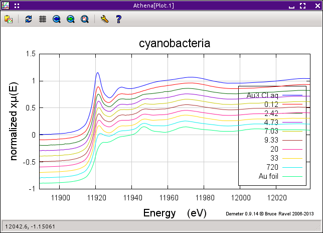
Fig. 12.14 The sequence of measurements from 0.12 through 720 hours. The top-most trace shows the starting material, aqueous Au³⁺ chloride. The bottom trace shows the end product, metallic gold.

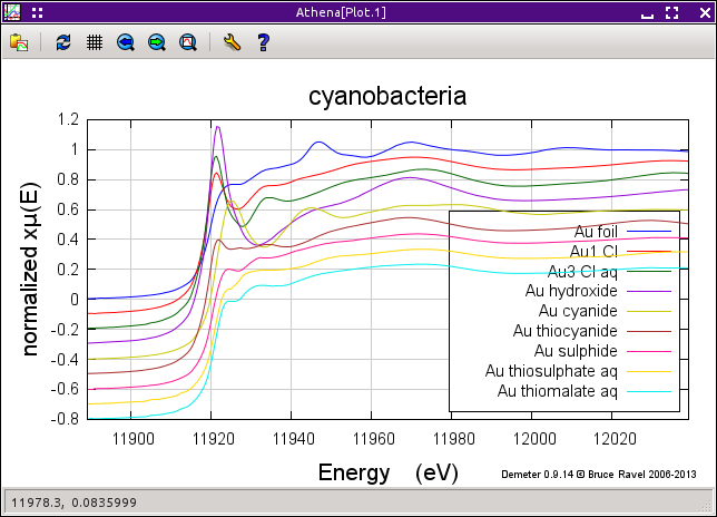
Fig. 12.15 All of the standards contained in the project file.

The purpose of this experiment is two-fold. One goal is to determine the reaction kinetics of the reduction. To that end, we will assume that the data are a linear combination of aqueous Au³⁺ chloride and metallic gold and measure their relative fractions as a function of time. The second goal is to determine whether the reduction involves an intermediate state and, if so, to identify that species. Our strategy to answer that question will involve adding other standard compound to our mixture of aqueous Au³⁺ chloride and metallic gold to see if the data are better described by a ternary rather than binary mixture of standard materials.

To begin, select one of the time points in the group list. Most figures in this section show the data measured at 7.03 hours. Next, select Linear combination fit from the main menu. This replaces the main window with the linear combination fitting tool and plots the data along with vertical lines indicating the extent of the fitting range. From the first two drop-down menus, select Au foil and Au3 Cl aq, as shown below.

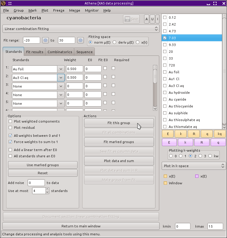
Fig. 12.16 The linear combination fitting tool with the end member standard compounds selected for the initial fit.

In the operations list, click on Fit this group to perform the initial fit to these data. After the fit finishes, the result of the fit, shown below is plotted. The tab labeled Fit results becomes active. Clicking on it, we see that the fit tells us that the data are 51±1 percent metallic gold. Given the quality of the fit, it seems that we are well justified in our assumption that these data can be modeled by a simple linear combination of the end members.

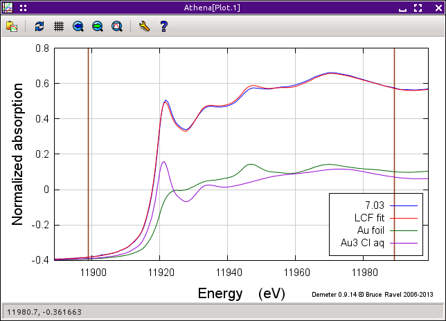
Fig. 12.17 The result of the initial fit to the 7.03 hour data using the end members as the fitting standards.

12.2.3. Improving the fit

As nice as this quick and easy result is, it's not perfect. A close examination of the plot above shows quite a bit of misfit throughout the entire fitting range. (Note that you can examine the misfit by clicking the Plot difference button and replotting the data by clicking Plot data + sum in the operations list.) This misfit suggests that our hypothesis of an intermediate state between Au³⁺ chloride and metallic gold may be valid.

As a first guess for what that intermediate state might be, I think should be something without a strong white line. The fit in the region of the white line is pretty good. Looking at the various standards on the right side of the first figure on this page I suspect that the sulfur ligated species, Au sulfide, Au thiosulfate, or Au thiomalate, are likely candidates. To test one, we need to add it to the list of fitting standards on the Standards spectra tab and rerun the fit. In the third row, select Au sulfide from the drop-down menu, then click Fit this group from the operations list.

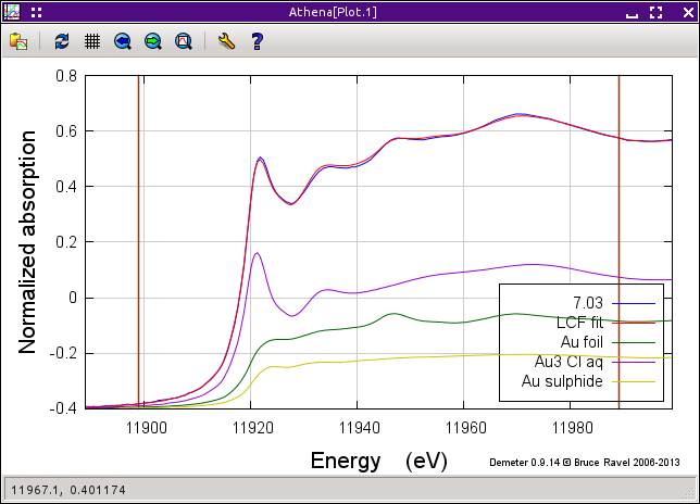
Fig. 12.18 The result of the fit to the 7.03 hour data using the end members along with gold sulfide.

This is a noticeably better fit. The amount of misfit throughout the fitting range and especially in the peak at about 11946.7 eV is smaller. Examining the results tab, we see that the amount of Au³⁺ chloride is about the same as before but that the metallic gold content is only 34±2 percent, with the sulfide taking up the remaining 18±2 percent.

12.2.4. Understanding the fit

The fit including the sulfide certainly looks better, but is it? The results tab also reports some simple statistics from the fit. The R-factor – a measure of mean square sum of the misfit at each data point – was 0.000073 for the two-standard fit and shrank by a factor of 2 to 0.000035 for the three-standard fit. That confirms the observation that the degree of misfit seems smaller in the plot of the three-standard fit.

The reduced χ² of the fit also reduced by about a factor of two, from 0.0000514 to 0.0000250, suggesting a substantive improvement in the fit quality. Those are strange numbers, though. Any textbook on scientific statistics will tell us that a good fit using a non-linear, least-squares minimization (such as that used by IFEFFIT and ATHENA) should give 1 for a fit in which the model is a good representation of the data. That is certainly true, but supposes that you have a good determination of the measurement uncertainty. We don't. In principle, the standard deviation spectrum from the merge of measured data could be used as an approximation of the measurement uncertainty, but that is not possible in this case. The data at 7.03 hours are a single measurement from a time sequence. There is nothing to merge because each measurement is a solitary measurement. Consequently, ATHENA has to use 1 as the value of the measurement uncertainty. That is grossly in excess of the true measurement uncertainty, resulting in very small values for χ².

We cannot, therefore, assert that any particular fit is a good fit simply by invoking what we know about Gaussian statistics. We can, however, compare successive fits, such as the two we have made thus far. An improvement of a factor of 2 in the value of reduced χ² is certainly significant. We can, with confidence, state that there is an intermediate component on the basis of the analysis presented thus far.

But what is that intermediate. We have not yet proven its identity (although gold sulfide is a strong contender!) because we have not yet considered other options. There are two algorithmically distinct but conceptually identical ways to attempt to solve this problem. One involves the use of principle component analysis (a feature not yet available in ATHENA) of the data followed by target transform analysis to attempt to identify the third species from among the standards. The approach discussed here involves using combinatorial techniques to directly test a library of standards against our data.

The mathematics of these two approaches is quite different. Since they share one major limitation, they are practically equivalent ways of identifying the intermediate state. The limitation is that both approaches require that the intermediate species be represented by the library of standards. If that unknown species is absent from the library, neither technique is able to identify it.

12.2.5. Combinatorial analysis

Testing each standard against the data sounds like an unbearably boring process – particularly since we may, in principle, want to consider all possible binary, ternary, or higher combinations of standards. The project file contains 9 standards. All possible combinations of 2 or 3 standards from a pool of 9 results in 120 possibilities. Performing and recording the results from that many fits sounds horrible. Fortunately, ATHENA knows how to automate that chore.

First mark all of the standards and none of the cyanobacteria data. Then click the Use marked groups button. This will insert all of the standards into the table.

By default, the table is only four rows long. You will need to exit the linear combination fitting tool and open the preference tool. Set the ♦Linearcombo→maxspectra preference to at least 9. Return to the linear combination tool and load the 9 standards into the table.

Click the Use at most control down to three. At this point you could click Fit all combinations to begin fitting all 120 combinations of 2 and 3 standards. This is, however, a bit of a waste of time. We know that there is metallic gold in these data. The fifth column in the table of standards is labeled req., which is short for required. Click the radiobutton in the Au foil row. This will cause the combinatorial sequence to only consider combinations which include the metallic gold standard. This reduces the number of binary and ternary combinations to 36. Now click Fit all combinations in the operations list. This will take a while. It's a good time to get that cup of coffee.

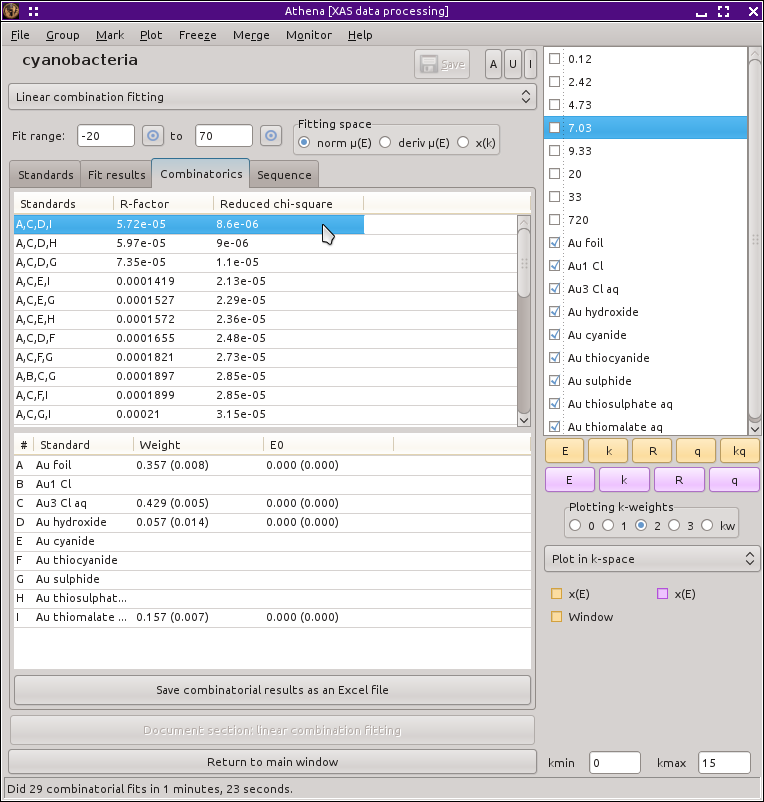
Fig. 12.19 The results of the combinatorial fitting sequence, as displayed on the in the combinatorics tab.

Once the sequence of fits finishes, ATHENA displays tables containing the results of all of the fits in order of increasing R-factor. The first column of the top table shows which standards were included in the fits using the numbering scheme of the bottom table. The other two columns show the R-factor and reduced χ² of each fit.

When you click on a row in the top table, the results of that fit are inserted into the bottom table and the fit is plotted. When the combinatorial sequence finishes, the best fit of the bunch is displayed. It turns out the the combination of gold metal, aqueous Au³⁺ chloride, and gold sulfide that we examined above is, in fact, the best fit. However, it is juts barely the best fit. The fit with gold thiomalate in place of gold sulfide is just barely worse. From a statistical perspective, the two fits are equivalent and the amounts of metal and chloride in the fits are very similar. The gold thiosulfate and gold thiocyanide fits are just a bit worse yet. A couple of other fits show similar statistics but an investigation shows that the peak around 11946.7 eV is not fit very well. After that, the other fits in the table fall off quickly in quality.

The conclusion that one can comfortably draw from this is that the intermediate species is some sort of gold-sulfur complex. The aqueous gold sulfide standard gave the best result by a hair, but the other three species with a gold-sulfur ligand were statistically similar. To model the kinetics in this system, I will use the sulfide species, but it is probably not correct to say that the intermediate species is aqueous gold sulfide. Rather it is some gold-sulfur complex formed when the cyanobacteria bacteria cells lyse upon exposure to the Au³⁺ chloride solution.

12.2.6. Analyzing the data series

To investigate the kinetics of this system, we will now apply the model consisting of three species – metal, chloride, and sulfide – to the cyanobacteria measured at each time step. Click on the top line of the upper table. This will plot the result for our best fit. It will also insert those three standards into the table on the Standards spectra tab. Click on that tab, then mark all the cyanobacteria data groups and unmark all of the standards in the group list. Now click on Fit marked groups in the operations list. This will step through the marked groups, applying the three-standard fitting model to each one. Again, you may want to relax as you wait.

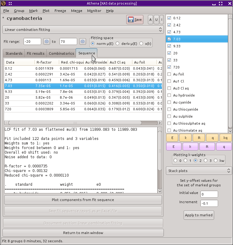
Fig. 12.20 A report on the results of fitting the marked groups. The report is written to a file that can be imported into a spreadsheet, like LibreOffice Calc shown here.

Once the sequence of fits finishes, you may want to click through the data groups and examine the fits at the various time steps. Note that the Marked fits report option in the operations list becomes active. Clicking on this prompts you for a name for an output file. This output file is a comma separated value text file which can be easily imported into a spreadsheet, much like one of ATHENA's report files. In this figure we see that the metal content increases monotonically while the chloride content decreases monotonically. The column with the sulfide content is not seen in the image, but it remains roughly constant throughout the experiment.

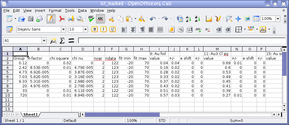
Fig. 12.21 A report on the results of fitting the marked groups. The report is written to a file that can be imported into a spreadsheet, like LibreOffice Calc shown here.

In this example, I have outlined the analysis performed in the paper cited at the beginning of the chapter. We have, as we set out to do, examined the reaction kinetics and tentatively identified an intermediate species. Using automation built right into ATHENA it was relatively easy to manage a large quantity of data.

---

DEMETER is copyright © 2009-2016 Bruce Ravel – This document is copyright © 2016 Bruce Ravel

This document is licensed under The Creative Commons Attribution-ShareAlike License.

If DEMETER and this document are useful to you, please consider supporting The Creative Commons.