13.2. Example 2: Methyltin¶

Some years ago, some colleagues from the U.S. Environmental Protection Agency came to me with an interesting problem about the fate and transport of organic tin compounds through sewage systems. In the U.S. (and elsewhere), municipal water is carried into homes and office buildings with copper pipes and waste water is transported to the water treatment system in polyvinyl chloride (PVC) pipes. By itself, PVC is a highly malleable plastic. Like many plastics, it is made stiff by the addition of stiffening agents added to the plastic matrix. In the case of PVC, organic tin compounds are used.

The folks from the EPA were studying the accumulation of tin in municipal waste and trying to understand if there was a mechanism of transport involving leaching from PVC pipes. We made a series of XAS measurements on various organic tin standards as well as direct measurement of PVC pipes produced by three different manufacturers.

Christopher A. Impellitteri, Otis Evans, and Bruce Ravel. Speciation of organotins in polyvinyl chloride pipe via X-ray absorption spectroscopy and in leachates using GC-PFPD after derivatisation. J. Environ. Monit., 9:358–365, 2007. doi:10.1039/B617711E.

Two of the standard compounds we measured were methyltin chloride, as shown below.

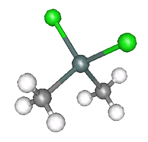
Fig. 13.15 Dimethyltin dichloride – one tin atom with two carbon ligands (in the form of methyl groups) and two chlorine ligands.

../_images/monomethyltin_trichloride.png

Fig. 13.16 Monomethyltin trichloride – one tin atom with two carbon ligands and two chlorine ligands.

These samples were prepared in solution. This solution was packed into a simple transmission sample cell for liquids. Transmission EXAFS were measured. Here is the data:

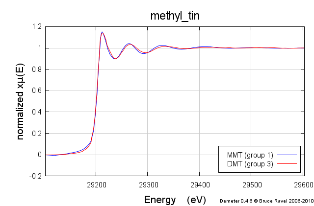
Fig. 13.17 μ(E) data measured on the dimethyltin dichloride and monomethyltin trichloride.

Fig. 13.18 χ(k) data measured on the dimethyltin dichloride and monomethyltin trichloride.

Fig. 13.19 χ(R) data measured on the dimethyltin dichloride and monomethyltin trichloride.

These data are quite similar, but there is a distinct change in the χ(R) spectrum between the two.

In this section, we will step through the corefinement of these two data steps, creating a constrained fitting model that uses the information content of both data sets to allows excellent measurement of a number of structural parameters.

You can find example EXAFS data and a structure from which to build the feff.inp file at my XAS Education site. Import the μ(E) data into ATHENA. When you are content with the processing of the data, save an ATHENA project file and dive into this example.

13.2.1. Import data¶

After starting ARTEMIS, leftclick click on the Add button at the top of the Data sets list in the Main window. This will open a file selection dialog. Click to find the ATHENA project file containing the data you want to analyze. Opening that project file displays the project selection dialog.

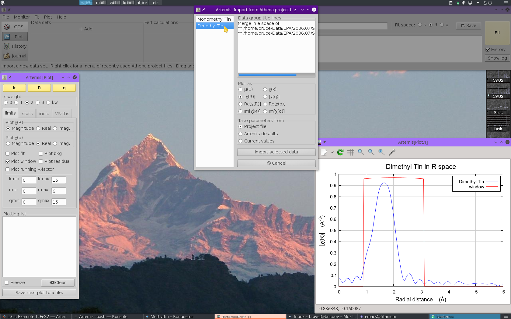
Fig. 13.20 Import data into ARTEMIS

The project file used here has the data from both methyltin standards. Select “Dimethyl Tin” from the list. That data set gets plotted when selected.

Now leftclick click the Import button. That data set gets imported into ARTEMIS. An entry for the dimethyl tin is created in the Data list, a window for interacting with the dimethyl tin data is created, and the dimethyl tin data are plotted as χ(k).

The next step is to import some structural data that can be used to make the FEFF calculation. Since this is a solution standard, there is obviously not an atoms.inp file. So we need to find another way to create the feff.inp file.

A bit of searching on Google eventually turned up the following structural information for dimethyltin dichloride in the form of a Protein Data Bank file. PDB is a format that is usually used to store structural data for large macromolecules, but is also quite suitable to tiny molecules like our methyl tin sample. This example has some chaff that is not of interest to us for our EXAFS analysis problem, but among the chaff is all the information we need.

COMPND    5261536
HETATM    1  C1  LIG     1      -0.027   2.146   0.014  1.00  0.00
HETATM    2 SN2  LIG     1       0.002  -0.004   0.002  1.00  0.00
HETATM    3  C3  LIG     1       1.042  -0.716   1.744  1.00  0.00
HETATM    4 CL4  LIG     1      -2.212  -0.821   0.019  1.00  0.00
HETATM    5 CL5  LIG     1       1.107  -0.765  -1.940  1.00  0.00
HETATM    6 1H1  LIG     1       0.996   2.523   0.006  1.00  0.00
HETATM    7 2H1  LIG     1      -0.554   2.507  -0.869  1.00  0.00
HETATM    8 3H1  LIG     1      -0.537   2.497   0.911  1.00  0.00
HETATM    9 1H3  LIG     1       0.532  -0.365   2.641  1.00  0.00
HETATM   10 2H3  LIG     1       1.057  -1.806   1.738  1.00  0.00
HETATM   11 3H3  LIG     1       2.065  -0.339   1.736  1.00  0.00
END

Note that columns 6, 7, and 8 contain the Cartesian coordinates of the tin, chlorine, carbon, and hydrogen atoms that make up the dimethyltin dichloride molecule. The third column identifies which atomic species lives at each of the sites. Perfect!

A bit of cutting and pasting into en empty template for a feff.inp file, resulted in the following:

TITLE dimethyltin dichloride

HOLE 1   1.0   *  Sn K edge  (29200.0 eV), second number is S0^2

*         mphase,mpath,mfeff,mchi
CONTROL   1      1     1     1
PRINT     1      0     0     0

RMAX        6.0

*CRITERIA     curved   plane
*DEBYE        temp     debye-temp
NLEG         4

POTENTIALS
*    ipot   Z  element
      0   50   Sn
      1   17   Cl
      2    6   C
      3    1   H

ATOMS
*   x          y          z      ipot  tag              distance
  -0.027   2.146   0.014  2
   0.002  -0.004   0.002  0
   1.042  -0.716   1.744  2
  -2.212  -0.821   0.019  1
   1.107  -0.765  -1.940  1
   0.996   2.523   0.006  3
  -0.554   2.507  -0.869  3
  -0.537   2.497   0.911  3
   0.532  -0.365   2.641  3
   1.057  -1.806   1.738  3
   2.065  -0.339   1.736  3

This was saved to disk, then imported into ARTEMIS by leftclick left clicking on the line in the Data window that says Import crystal data or a Feff calculation, then selecting our feff.inp file from the column selection dialog.

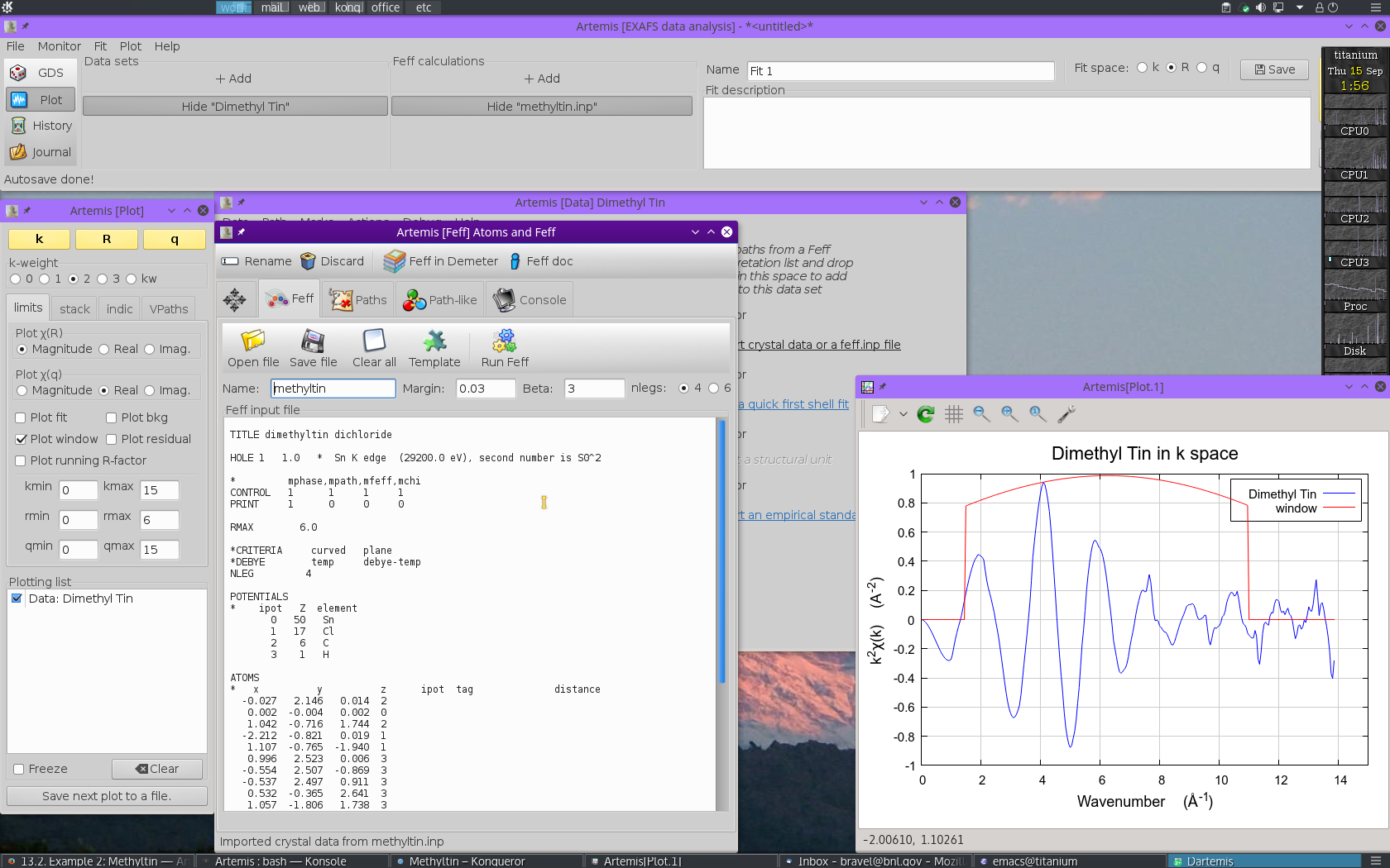
Fig. 13.21 Importing information for making the FEFF calculation.

With the methyltin structural data imported, run FEFF by leftclick clicking the Run Feff button to compute the scattering potentials and to run the pathfinder.

Once the FEFF calculation is finished, the path intepretation list is shown in the Paths tab. This is the list of scattering paths, sorted by increasing path length. Select the first 2 paths by leftclick clicking on the path 0000, then Control- clicking on path 0002. The selected paths will be highlighted. Click on one of the highlighted paths and, without letting go of the mouse button, drag drag the paths over to the Data window and drop them onto the empty Path list.

Fig. 13.22 drag Drag and drop paths onto a data set

drag Dropping the paths on the Path list will associate those paths with that data set. That is, that group of paths is now available to be used in the fitting model for understanding the methyltin data.

Each path will get its own Path page. The Path page for a path is displayed when that path is clicked upon in the Path list. Shown below is the dimethyltin dichloride data with 2 paths. The first path in the list, the one representing the contribution to the EXAFS from the C single scattering path nominally at 2.150 Å, is currently displayed. The second path represents the contribution to the EXAFS from the Cl single scattering path nominally at 2.360 Å.

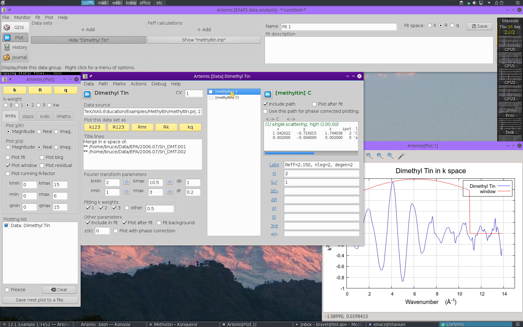
Fig. 13.23 Paths associated with a data set

13.2.2. Examine the scattering paths¶

The first chore is to understand how these two paths from the FEFF calculation relate to the data. To this end, we need to populate the Plotting list with data and paths and make some plots.

Mark single scattring paths for the C and Cl by leftclick clicking on their check buttons. Transfer those two paths to the Plotting list by selecting Actions ‣ Transfer marked.

With the Plotting list poluated as shown below, leftclick click on the R plot button in the Plot window to make the plot shown.

Fig. 13.24 Methyltin data plotted with the first four single scattering paths

These two paths reasonably might represent the peak in the dimethyltin dichloride data, although it is not clear how the lower part of that peak will be represented by these two paths. It is instructive also to look at the data as the real part of the Fourier transform. To do so, leftclick click the Real radiobutton under Plotχ(R) in the Plotting window. This will display the following plot:

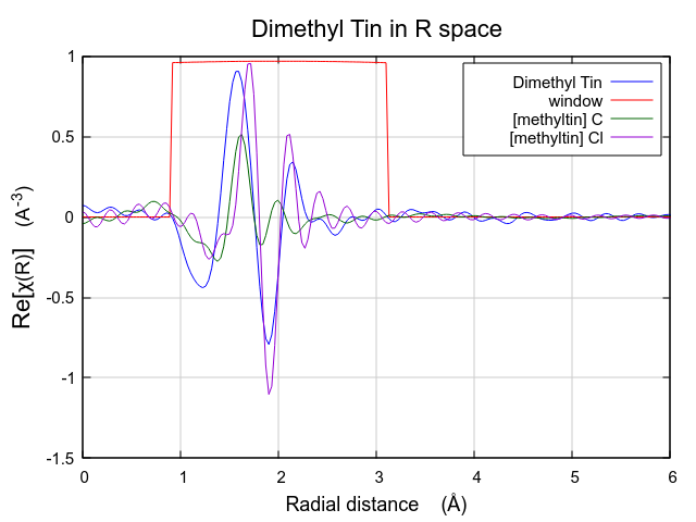
Fig. 13.25 The data and two paths, plotted as Re[χ(R)].

Viewed this way, it is clear that this FEFF calculation is likely to do a good job fitting these data. The missing spectral weight at low R could likely be recovered by a ΔR shift of the the C scatterer to lower R.

13.2.3. Fit to the dimethyltin dichloride data¶

As in many fits, we will use a single parameter to represent the S²₀ for each path. This is reasonable as this is a parameter of the absorber and we are making only one FEFF calculation in this fit. For the same reason, we will use a single E₀ parameter for each path. We don't have any a priori knowledge of how the Sn-C and Sn-Cl bonds might be related. As a result, we will float independent ΔR and σ² for the two ligands. This results in 6 fitting parameters.

Make sure both the C and Cl paths are included in the fit. That is, each should have its Include path button checked.
Set the values of R_min and R_max to cover just the first peak. 1 Å to 2.4 Å is a good choice.
We need parameters to represent S²₀ and E₀. The parameters amp and enot are defined in the GDS window and given sensible initial guess values.
We need ΔR and σ² for each ligand type. The ΔR parameters are called drc and drcl. The σ² are called ssc and sscl.

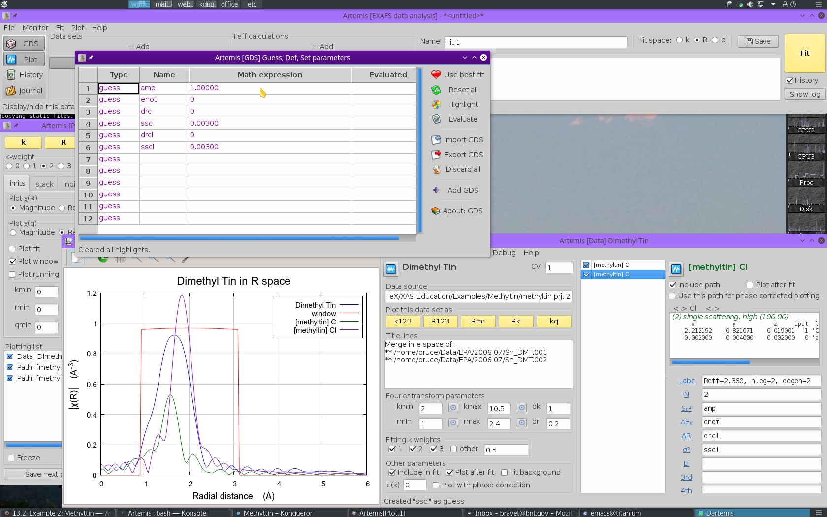
Fig. 13.26 Six parameters are defined and used as path parameters.

At this point we are ready to leftclick click the big fit button. Doing so yields the following:

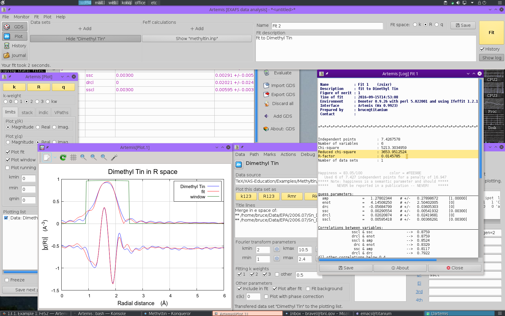
Fig. 13.27 Fit to the dimethyltin dichloride data using the simple, 6-parameter fitting model.

Glancing at the plot window, this looks like a decent enough fit. Examining the log file, we find that the fit is fairly well interpretable.

The S²₀ value is 1.27±0.28, which is rather larger than expected
E₀ is 4.1±2.5 eV, a reasonable value which suggests that E₀ was chosen reasonably in ATHENA.
As expected, ΔR for the C ligand is negative and fairly large at -0.057±0.036 Å. The ΔR for the Cl ligand is positive, but consistent with zero, 0.020±0.024 Å.
Both σ² values are of a reasonable size, 0.00291±0.00542 Å² for C and 0.00595±0.00366 Å² for Cl.

Note, however, that the information content of this fit is being heavily strained. With a k-range of 2 Å^-1 to 10.5 Å^-1 and an R-range of 1 Å to 2.4 Å, there are only about 7.4 independent measurements in these data. The six parameters floated in this fit are a significant burden on these data.

13.2.4. The benefit of multiple k-weight fitting¶

Before extending this fitting project to consider corefinement of the two methyltin data sets, let us pause and consider the merits of multiple k-weight fitting.

The default in ARTEMIS is to perform the fit with k-weighting of 1, 2, and 3. The implementation of this is quite simple. The normal χ² fitting metric is evaluated for each value of k-weighting considered. The sum of all these χ² evaluations is then minimized to produce the fit. The advantage of doing this can be seen when considering the impact of the various path parameters on the EXAFS equation.

A σ² parameter is always multiplied by k² in the EXAFS equation. Thus the portion of the fitting metric evaluated at high k is much more sensitive to a poorly chosen value of σ² than the portion evaluated at low k. Since a k-weighting of 3 amplifies the value of the data (and theory) more and more as k increases, evaluating the fit with a k-weight of 3 will provide more sensitivity to σ² parameters. The other amplitude parameter, S²₀, affects all regions of the k-range equally.

Similarly, ΔR is multiplied by k in the EXAFS equation, thus the evaluation of the fitting metric at high k is much more sensitive to a poorly chosen value. E₀, on the other hand, has a much bigger impact on the evaluation of the fitting metric at low k. Thus a k-weight of 3 will provide greater sensitivity to ΔR in the fit while a k-weight of 1 will provide a greater sensitivity to E₀.

One might think, then, that a k-weight of 2 would be a good compromise between the demands of the various parameters. Let's check that out.

To perform a fit with just k-weight of 2, leftclick unclick the 1 and 3 buttons as shown in Fig. 13.28.

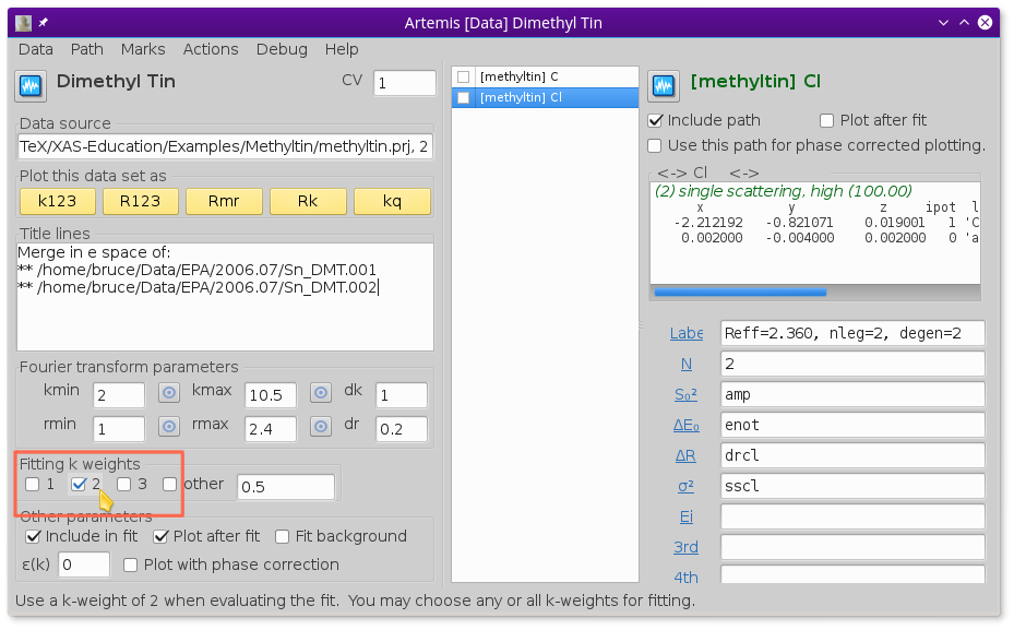
Fig. 13.28 Changing the fitting k-weight so that the fit is made only with k-weight equal to 2.

We leftclick click the big fit button and a minute later we see this:

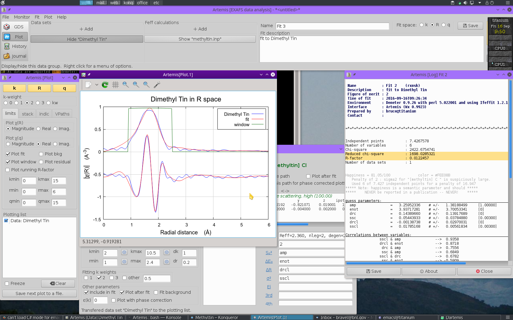
Fig. 13.29 The result of the fit using k-weight of 2.

On the surface, this appears to be a comparable fit to the one made with multiple k-weighting. The quality of the plot is similar, as is the value of R-factor. Closer examination of the fitting parameters turns up a number of serious problems.

The value of S²₀ is 3.26±1.38! The result with multiple k-weight fitting was also greater than 1, but could possibly be explained as a problem of sample preparation or mean free path. This value is just nonphysically enormous.
To compensate for the large S²₀, the values for σ² are also unreasonably large, 0.05444±0.03785 Å² for C and 0.01785±0.00562 Å² for Cl.

The effect of these hard-to-understand values for S²₀ and σ² can be seen in Fig. 13.31. Both contributions are very broad, as expected given their large values for σ². This is in contrast to the contributions from the multiple k-weight fit shown in Fig. 13.30, where they are of a width that seems more reasonable for tightly bound ligands.

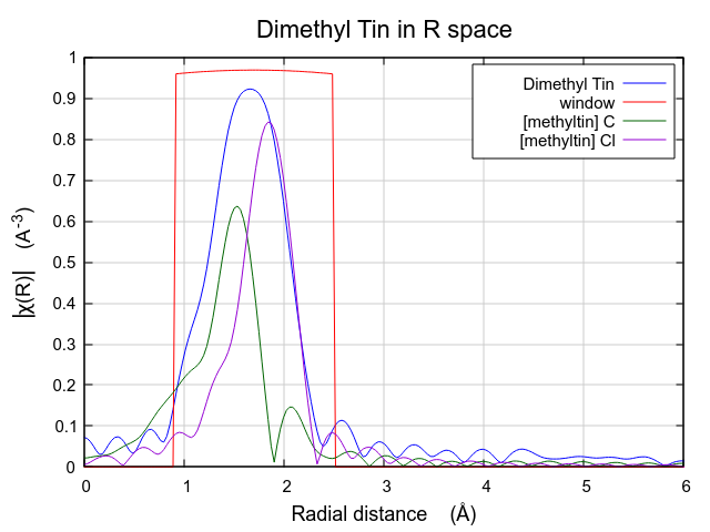
Fig. 13.30 The C and Cl contributions to the multiple k-weight fit.

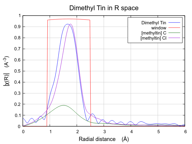
Fig. 13.31 The C and Cl contributions to the fit using k-weight of 2.

In this situation, where the number of guess parameters is such a large fraction of the total information content of the data, the use of multiple k-weight fitting is essential. The added sensitivity to the various regions of k-space afforded by the evaluation of the fitting metric with different k-weight values helps reduce the very high correlations between the S²₀ and σ² parameters, resulting in a much more defensible fit.

13.2.5. Corefining multiple data sets¶

The solution to the problem of the number of guess parameters being so close to the number of independent points is to expand the bandwidth of the data. This is often done by extending the fitting model to include higher coordination shells, then importing and parameterizing additional FEFF paths to account for the structure at higher R. In this case, that will not work. These data have very little structure beyond about 2.5 Å. In this case, what we have fit so far is all there is to the data.

Another way of increasing the information content is to corefine multiple data sets. Adding a second data can double the information content of the fitting model. If the fitting model can be made to accommodate the new data set without doubling the number of guess parameters, the model should be more robust.

In this case, we will double the information content by adding the monomethyltin trichloride to the project – both methyltin data sets were measured over the same k-range and consist of a single peak in R. If we assume that the sate of the Sn atom is the same in both materials and we take care to align the data well in ATHENA, then we will not need to introduce new parameters for S²₀ or E₀.

If we further assume that the nature of the Sn-C and Sn-Cl bonds are very similar in the two forms of methyltin, then we can reuse the ΔR and σ² parameters for the C and Cl scatterers.

Thus we can double the information content of the fit while adding no new parameters!

To start, use the file selection dialog to again open the ATHENA project file containing the methyltin data. Select the monomethyltin data. This will import the second data set, add it to the Data sets list in the main window, and create a Data window for monomethyltin. All of this is shown in Fig. 13.32.

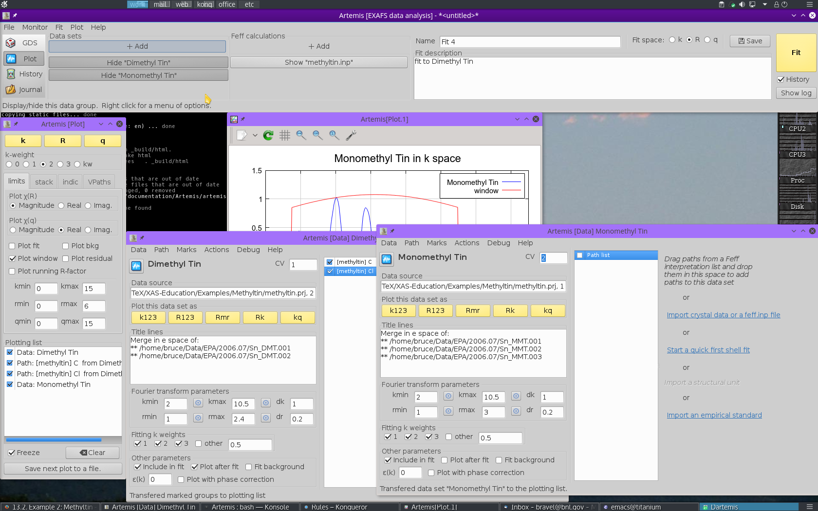
Fig. 13.32 Importing the monomethyltin trichloride data into the fitting project.

Re-open the window containing the FEFF calculation, then drag drag and drop the same two paths onto the monomethyltin window.

Fig. 13.33 Reuse the guess parameters from before, but change the coordination numbers for C and Cl to 1 and 3, respectively.

Edit the path parameters so that the paths in the new monomethyltin window use the same parameters for S²₀, E₀, ΔR, and σ² as were used for the dimethyltin.

To account for the different numbers of C and Cl ligands, the N path parameters must be changed to 1 for C in the dimethyltin data window and 3 for the Cl.

Make sure the R-range is set sensibly. You are now ready to hit the big fit button.

Fig. 13.34 The data and fitted paths for the multiple data set fit to the dimethyltin and monomethyltin data.

Fig. 13.35 The log file from the multiple data set fit to the dimethyltin and monomethyltin data.

This is a decent fit. The guess parameters are mostly reasonable, although the S²₀ parameter is still somewhat large. E₀, ΔR, and σ² values are all defensible. The uncertainties on most of the parameters are smaller than in earlier fits. Most importantly, we are not stressing the information content of the data so severely by fitting 6 parameters.

My having more unused information available, we can explore other possibilities in these data that would not have been possible in the single data set fit. For example, we could examine the impact of the H single scattering paths on the fit or we could try lifting the constrains on the ΔR and σ² parameters of the two ligand types.

13.2.6. Further exploration¶

Could the Fourier transform range be longer? Look at the k123 plot for each data set.
Could the fitting range be longer? Well, there is not much signal beyond the first shell above the noise level. Simply expanding the R-range to make N_idp larger without actually including signal is cheating.
Is the assumption about the bonds in the two samples valid? How would you go about testing that assumption?
Trimethyltin monochloride would have been a useful measurement....
The ΔRs for both Sn-C and the Sn-Cl are somewhat large. The fit might be improved by adjusting the original feff.inp, re-running FEFF, and re-doing the fit.
The structure used in the FEFF calculation is unbounded from the outside, which might effect the construction of muffin tins. Packing water molecules around the DMT molecule might help.
Is the dimethyltin feff calculation really transferable to monomethyltin? You could test this by finding or creating a structure for monomethyltin trichloride and running FEFF on that.

This document is licensed under The Creative Commons Attribution-ShareAlike License.

If DEMETER and this document are useful to you, please consider supporting The Creative Commons.