4.3. The Paths tab
When you click the Run Feff button on the FEFF tab, the FEFF calculation is run. Once finished, a succinct summary of the calculation is displayed on the Paths tab.

Fig. 4.6 The Paths tab.
Some statistics about the FEFF calculation are shown in the Description text box. Below that is the summary of the paths found in the FEFF calculation. This summary is presented in the form of a table. Each row describes a scattering path. The columns contain the following information:
- The first column shows a path index, similar to the index that FEFF uses when run by hand from the command line.
- The second column shows the degeneracy of the path.
- The third column shows its nominal path length, Reff. That
is value that will be used in any path parameter math
expression containing the
refftoken. - The fourth column shows a simple view of the scattering path. The
@token represents the absorber, thus appears as the first and last token in each description. The tokens representing the scattering atoms are taken from the tags on the FEFF tab. You can change the absorber token by setting the ♦Pathfinder→token configuration parameter. - The fifth column contains the rank of the path. This is an attempt to predict how important of each path will be to your fitting model. Paths with large spectral weight have a large rank and paths with little spectral weight have small rank. Highly ranked paths are colored green, mid-rank paths are colored yellow, and low-rank paths are grey. Don't put too much faith in this assessment of importance. You should explicitly check all paths to decide if they should be included in a fit.
- The sixth column gives the number of legs in each path.
- The final column is a simple explanation of the shape of the scattering geometry.
The rows in this table are selectable by mouse
click.  Left clicking on a row selects that
row. Control- clicking on another row
adds it to the selection. Shift-
clicking adds to the selection all rows between the one clicked upon
and the previously clicked upon row.
Left clicking on a row selects that
row. Control- clicking on another row
adds it to the selection. Shift-
clicking adds to the selection all rows between the one clicked upon
and the previously clicked upon row.
Much of the functionality of this page rests upon the set of selected paths. Most importantly, selecting paths is the first step to using paths in a fitting model. This will be explained in the next chapter.
At the top of the page is a bar of buttons used to perform tasks specific to the path list. The Doc button will open a browser displaying this documentation for the interpretation page. The Rank button is described below. The remaining buttons are related to making plots of the selected paths.
4.3.1. Polarization
If FEFF has been run considering linear polarization, the path list may be considerably longer. The degeneracy checker in the path finder calculation will recognize the effect of polarization on path degeneracy. Paths with common outgoing and incoming angles of the photoelectron with respect to the specified polarization vector will be treated as degenerate. Paths which would be degenerate in the absence of polarization, but which have distinct outgoing and/or incoming angles will be presented as separate paths in the path list.
When the polarization calculation is performed, the outgoing and incoming angles will be displayed in Scattering path column (although you may need to widen the column by clicking on and dragging the little vertical line that separates the Scattering path and Rank columns in the header row).
Also, when  dragging a path onto the data page, the
angles out and in will be displayed in the path geometry box on the
path page.
dragging a path onto the data page, the
angles out and in will be displayed in the path geometry box on the
path page.
Optionally, the angles can be displayed in the path list label by setting the ♦Pathfinder→label configuration parameter appropriately.
Low ranking paths are, by default, not displayed in the paths list. In a polarization calculation, typically, paths close to or at 90 degrees in either angle will have very small amplitude and so will not be displayed in the path list. This behavior of suppressing low-ranking paths can be controlled by setting the ♦Pathfinder→postcrit configuration parameter. Setting it to 0 will cause all paths, even the right angle ones, to be displayed in the paths list.
Caution
FEFF's ELLIPTICITY keyword is not
supported at this time. That means the trick of modeling
“polarization in the plane” is not yet supported by
ARTEMIS.
4.3.2. Path plotting and path geometry
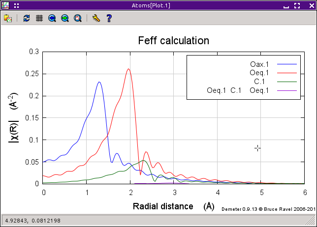
Fig. 4.7 This is a plot of paths from the raw Feff calculation.
In this example, the first three single scattering paths from the sodium uranyl triacetate calculation were selected along with a low-rank multiple scattering path. Then the Plot selection button was pressed. In this plot, we see that the three single scattering paths are, indeed, quite large. The multiple scattering path can barely be seen on this scale. It truly is a low importance path.
The meaning of a “raw” FEFF calculation is that it is displayed as χ(k) with S20 set to 1.0 and each of E0, ΔR, and σ2 set to 0. A plot of χ(R) for the “raw” FEFF calculation, then, displays the Fourier transform of χ(k) parameterized with those values.
It is, therefore, very quick and easy to examine the results of a FEFF calculation. The other four buttons are used to select how the plot of paths is made. The options are χ(k), | χ(R)|, Re[χ(R)], and Im[χ(R)]. The k-weight selected in the Plot window is used to make the plot of paths.
 Right clicking on an entry in the paths list
will post a menu. The first item on the menu opens a dialog window
with more details about the geomtery of the selected scattering
path. In the following figure, the selected path (0006) was
right-clicked on, opening the dialog depicted
below.
Right clicking on an entry in the paths list
will post a menu. The first item on the menu opens a dialog window
with more details about the geomtery of the selected scattering
path. In the following figure, the selected path (0006) was
right-clicked on, opening the dialog depicted
below.
The other context menu options are used to set the path select on the
basis of distance, ranking, or scattering geometry. These options are
useful for selecting groups of paths to drag and drop
onto the Data window.
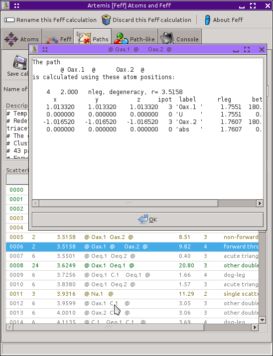
Fig. 4.8 Information about the geometry of a scattering path.
The contents of the path interpretation can be filtered after running the FEFF calculation by setting the ♦Pathfinder→postcrit parameter. By default, it is set to 3, which means that only paths with a ranking above 3 will be displayed in the path interpretation. Resetting this parameter allows you tune how many paths get displayed after the calculation.
4.3.3. Path ranking
FEFF provides a crude evaluation of the importance of each path called the “curved wave importance factor”. This is computed as a very sparse – computed at four points between 0 Å-1 and 20Å-1 – trapezoidal integration of | χ(k)|. This amplitude is then expressed as a percentage with the largest path having an amplitude of 100.
There are a few shortcomings of FEFF's amplitude factor. First, the percentages are computed serially. So the first path is always given as 100%. If a subsequent path is larger than the first path, it, so, will be given as 100%. All following paths will be scaled to size of the later path. This is somewhat confusing.
Second, the integration is very sparse. This made sense back in the mid-90s, when computers were slower and had less memory. But it means the amplitude is not very accurate.
Finally, the integration is over a much wider range in k-space than is typically measured in a real experiment. It would make more sense to evaluate a measure of the importance of a path over a range in k that is expressed in a real measurement or, at least, a range that is more typical of a normal experiment.
To this end, ARTEMIS offers a variety of new ways to rank the importance of a path. Some use χ(k) and some use χ(R) of the paths. All are evaluated over a restricted range in k or R. By default, the range in k is 3Å-1 and 12Å-1 and in R it is 1 Å and 4 Å. All are evaluated using the full k or R grid which is used internally. Some consider k-weighting.
They all have funny acronyms:
- akc
- This is the sum over the k-range of the absolute value of k χ(k).
- aknc
- This is the sum over the k-range of the absolute value of knχ(k) where the plotting k-weight is used for n.
- sqkc
- This is the square root of the sum over the k-range of the square of k χ(k).
- sqknc
- This is the square root of the sum over the k-range of the square of knχ(k) where the plotting k-weight is used for n.
- mkc
- This is the sum over the k-range of k| χ(k)|.
- mknc
- This is the sum over the k-range of kn||chi| (k)| where the plotting k-weight is used for n.
- mft
- This is the maximum value of | χ(R)| within the R-range where the plotting k-weight is used for the Fourier transform.
- sft
- This is the sum over the R-range of | χ(R)| where the plotting k-weight is used for the Fourier transform.
These new ranking criteria tend to do a better job of correctly predicting which paths are important to a fit. That's a good thing. The bad thing is that they take quite a bit longer to compute than simply relying on FEFF's amplitude ratios.
The full suite of options are provided in order to replicate the analysis shown in the paper by K. Provost, et al. The “akc” and “aknc” choices tend to be reliable.
You can select which criterion to use on the interpretation page by setting the ♦Pathfinder→rank configuration parameter to feff or to one of the acronyms above.
You can compare the evaluations of the ranking criteria by pressing the Rank button in the toolbar. This calculation takes about a third of a second per path. If there are a lot of paths in the interpretation, this can be a bit time consuming. At the end, a text dialog with the various rankings for each path is displayed. As can be seen in the figure below, there is some variation between the criteria, but all of them differ substantially from FEFF's importance factors.
Fig. 4.9 The report on the path ranking calculation.
This improvement upon FEFF's path selection tool is adapted from
- K. Provost, B. Ravel, and A. Michelowicz. Improving the estimation of scattering paths amplitude for path selection in EXAFS fit. Application to bis(S-thiocyanato)(cyclohexanediamino)platinum(II). J. Synchrotron. Radiat., 2015. submitted.
None of the path ranking criteria currently use σ2 when they are being evaluated, but that would be an interesting consideration.
DEMETER is copyright © 2009-2016 Bruce Ravel – This document is copyright © 2016 Bruce Ravel
This document is licensed under The Creative Commons Attribution-ShareAlike License.
If DEMETER and this document are useful to you, please consider supporting The Creative Commons.