13. Hephaestus

In his workshop he has handmaidens he has forged out of gold
who can move and who help him in his work. ...  With Athena,
[Hephaestus is] important in the life of the city.  The two
[are] the patrons of handicrafts, the arts which along with
agriculture are the support of civilization.
                             Mythology, Edith Hamilton

HEPHAESTUS is a program for making small calculations useful to the XAS experimentalist using a periodic table, tables of X-ray absorption coefficients, and other elemental data.

To start HEPHAESTUS, double click on its icon or, at the command line, type dhephaestus (that's pronounced hə'fɪstəs, with a silent d).

On the left of the HEPHAESTUS window is a stack of icon buttons which are used to select the different tools. Clicking on one of the icon buttons enables that tool.

At the bottom of the HEPHAESTUS window is a status bar which HEPHAESTUS uses to convey information during the course of operation. Along with information about the most recently completed calculation, the status bar shows topical information. As the mouse passes over an element in the periodic table, the element name, symbol, and Z number are displayed. In the Absorption tool, clicking on an edge or line energy will display that energy in wavelength units in the status bar. In the Standards tool, some information about the plotted data is displayed in the status bar.

The Hephaestus menu in the menu bar provides another way of navigating between the tools. The mouse can be used, as can the keyboard. Alt-e, Alt-p and Alt-h post the Hephaestus, Plot, or Help menus. Control-1 through Control-9 change the display the various tools. Control-m displays the document in a web browser, while Control-c changes the display to the configuration tool.

13.1. Absorption

This is the start page for HEPHAESTUS and is used to display information about edge and line energies for the elements.

A periodic table is displayed atop three lists that will be filled in with data associated with an element. Clicking on an element in the periodic table displays data about that element.

The data table will be filled with some basic information about the element, including its name and Z number, its atomic weight, and bulk density under standard temperature and pressure. Beneath this table are two controls for determining the appropriate Z-1 or Z-2 filter to use in a fluorescence experiment. The Filter text box will be filled with the likeliest candidate for the element selected from the periodic table. This can be edited by hand. Clicking the Plot filter button will display a plot showing the relative locations of the edge energy, the dominant fluorescence lines, and the filter edge energy.

The Absorption edges table shows the value in eV of each edge associated with the element selected from the periodic table and the core-hole lifetime in eV of each edge. Clicking on a line in this table will display a message in the status bar giving the edge energy expressed in wavelength units and the core-hole lifetime expressed in approximate time units. Double-clicking on a line will highlight all fluorescence lines associated with that edge in the Fluorescence lines table.

The definition of the core-hole lifetime is discussed in the tabulation by Keski-Rahkonen and Krause. In short, it is a measure of the width of the absorption edge. High energy edges – Sn for example – are very broad and have large core-hole lifetimes (as measured in energy), while low energy edges are much sharper. The numbers used by HEPHAESTUS are the same as those used by FEFF and are taken from that reference.

• Olavi Keski-Rahkonen and Manfred O Krause. Total and partial atomic-level widths. Atomic Data and Nuclear Data Tables, 14(2):139–146, 1974. doi:10.1016/S0092-640X(74)80020-3.

The Fluorescence lines table shows the transitions and emission energies in eV of every line associated with the element selected from the periodic table. Also shown is the approximate strength, or branching ratio, of each line. The strengths for all lines associated with a particular edge will sum to 1. Clicking on a line in this table will display a message in the status bar giving the emission energy expressed in wavelength units.

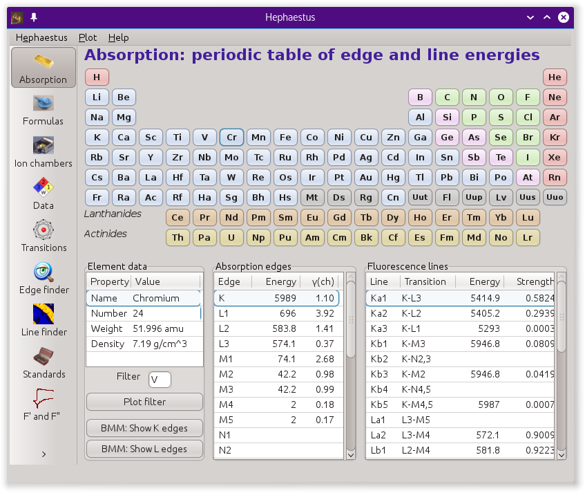
Fig. 13.1 The absorption tool.

13.1.1. Filters

The rules for the selection of the filter elements are:

1. For elements below Z=38, assume the K edge is being measured and use the Z-1 element.
2. For elements between Z=39 and Z=57, assume the K edge is being measured and use the Z-2 element.
3. Use Br for a Rb absorber because Kr is a silly filter material.
4. Use Rh for a Ru absorber because nobody wants a Tc filter!
5. Use I for a Ba absorber because Xe is also a silly filter material.
6. For elements above Z=57, assume the L_III edge is being measured. Use the first element whose K edge is more than 90 eV above the Lα₁ line of the absorber.
7. Use Rb for a U or Np absorber because Kr is still a silly filter material.
8. For elements below Z=24 (chromium), no filter choice is given. Filters for lower-Z elements are not used because no element exists with a K-edge between the line and absorption energies of the absorber.

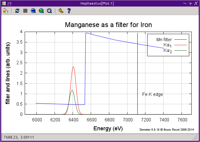
Fig. 13.2 A filter plot showing why manganese is a good choice for an iron absorber – it passes the fluorescence, which is below the Mn K edge, but preferentially absorbs the elastically scattered radiation.

13.1.2. Beamline customization

When beamline customization is enabled, the two buttons labeled Show K edges and Show L edges will be visible. These are both toggle buttons. When pressed, they will disable all elements that cannot be measured by that edge at the beamline.

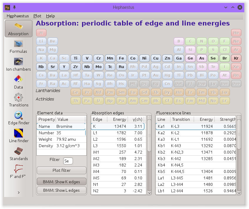
Fig. 13.3 The absorption tool with beamline customization for the NSLS-II BMM (6BM) beamline showing the elements whose K edges can be measured at the beamline.

To enable beamline customization, set the ♦Hephaestus→enable_beamline configuration parameter to true.

You will want to set the ♦Hephaestus→beamline_name parameter to the name of your beamline. Keep it short – it needs to fit on the button! Finally, set the ♦Hephaestus→beamline_emin and ♦Hephaestus→beamline_emax parameters to the lower and upper energy bounds of your beamline.

13.2. Formulas

This tool is used to compute approximate absorption lengths for common or user-specified materials. To the left is a list of materials commonly found at synchrotron beamlines. Clicking one of those items inserts its stoichiometric formula into the Formula box and the density into the Density box.

At the top of the right hand part of this tool are controls for entering the parameters of the absorption length calculation. The formula must be a stoichiometric formula using a few simple rules.

1. Element symbols must be first letter capitalized.
2. White space is unimportant – it will be removed from the string. So will dollar signs, underscores, and curly braces (in an attempt to handle TeX). Also a sequence like this: “/sub 3/” will be converted to “3” (in an attempt to handle INSPEC).
3. Numbers can be integers or floating point numbers. Things like 5, 0.5, 12.87, and .5 are all acceptable, as is exponential notation like 1e-2. Note that exponential notation must use a leading number to avoid confusion with element symbols. That is, 1e-2 is OK, but e-2 is not.
4. Uncapitalized symbols or unrecognized symbols will flag an error.
5. An error will be flagged if the number of open parentheses is different from the number of close parentheses.
6. An error will be flagged if any unusual symbols are found in the string.

The density is entered in units of specific gravity or grams per cubic centimeter. Alternately, units of molarity can be used by selecting that from the choice menu.

Finally, an energy in eV is required at which to make the calculation.

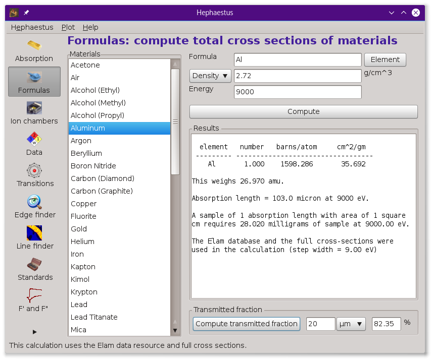
Fig. 13.4 The formulas tool.

At the bottom of the page is a tool for computing transmitted fraction from the material just computed. You can enter a sample thickness and choose from μm, m, and cm units. Pressing the Compute transmitted fraction button will use the cross section reported above to display the transmitted fraction of X-rays at the current energy through the sample. This is presented as a percentage of the incident intensity transmitted through the sample.

13.2.1. Detailed explanation

Here is an example of the results printed for BN, with a specific gravity of 2.29 and at energy of 7800 eV:

  element   number   barns/atom     cm^2/gm
 --------- ----------------------------------
    B        1.000  30.084        1.676
    N        1.000     123.417        5.306

This weighs 24.819 amu.

Absorption length = 0.077 cm at 7800 eV.

A sample of 1 absorption length with area of 1 square
cm requires 175.278 milligrams of sample at 7800.00 eV.

The Elam database and the full cross-sections were
used in the calculation.

This reports on an important physical parameter, the “absorption length”. This is defined as the length of sample over which the intensity of the incident beam will be attenuated by 1/e, or about 63%, at the specified energy. Note that absorption length is an energy dependent parameter and that it changes significantly across an absorption edge.

Here we see that 9000 eV photons will be e-fold attenuated in just over 1 millimeter of packed BN. To make a sample with an area of 1 square centimeter facing the beam and which has an absorption length of 1, one must weigh out about 175 milligrams of BN. In practice, this is quite a lot of BN and will make a rather thick pellet. One might weigh out a fraction of the 175 milligrams for a real sample, giving the matrix that much less than 1 absorption length.

As another example, here is the calculation on cobalt ferrite, CoFe₂O₄, which has a specific gravity of about 5. Computing the cross section at 7800 eV will trigger a calculation of the sample depth corresponding to a unit edge step at the Co K edge. This additional calculation is triggered because the calculation energy, 7800 eV, is within 100 eV of the Co K edge energy of 7709 eV.

  element   number   barns/atom     cm^2/gm
 --------- ----------------------------------
    Co       1.000   33808.991      345.519
    Fe       2.000   30183.487      325.464
    O        4.000     333.532       12.553

This weighs 234.633 amu.

Absorption length = 8.2 micron at 7800 eV.

A sample of 1 absorption length with area of 1 square
cm requires 4.079 milligrams of sample at 7800.00 eV.

Unit edge step length at Co K edge (7709.0 eV) is 28.3
microns

The Elam database and the full cross-sections were
used in the calculation.

Here we introduce a second important physical parameter, the “unit edge step length”. This is defined as the length over which the total absorption will change by a factor of 1/e as the incident beam energy is scanned over the absorption edge. To say that another way, the absorption will be e-fold greater just above the edge than just below the edge. With that length of sample, the edge step of a transmission XAS scan will be 1.

Suppose you wanted to mix some cobalt ferrite with 35 milligrams (i.e. an amount that will contribute 0.2 to the total absorption of the sample) of boron nitride measured above in order to make a good transmission XAS sample. That amount of BN contributes 0.2 absorption lengths to the total thickness of the sample at this energy. Weighing out 4 milligrams of ferrite, then, gives the sample a total absorption of 1.2. That is, the beam passing through the sample will attenuate to the level of exp(-1.2), or about 30%, of the intensity of the incident beam.

Note that this sample has more Fe than Co and that the calculation energy is above the Fe K edge energy. The Fe part of the sample is rather absorbing at this energy. As a result, a relatively small mass of sample constitutes an absorption length.

The 4 milligrams of sample required for one absorption length is distributed over 8.2 microns. The unit edge step calculation tells us that the edge step will be one with 28.3 microns of sample. Thus, the sample with one absorption length of ferrite will have an edge step of 8.2/28.3 = 0.34.

A sample with an edge step of 1 is made by mixing 28.3 milligrams of ferrite with the BN. This sample, however, will be rather thick around the Co K edge. 28.3 milligrams represents 2.9 (= 1/0.34) absorption lengths of ferrite. The ferrite in BN will, therefore, attenuate the beam passing through the sample to the level of exp(-3.1), or about 4.5%.

In an early XAS paper by Stern and Kim, it was shown that the edge step of a sample should not exceed 1.5. Using a simple statistical argument that presumes that measurement uncertainty is dominated by shot noise, the authors show that a sample is optimized when the total absorption is 2.6. In this case, the sample of ferrite in BN can be made such that both total absorption and edge step are close to optimal. For instance, making the sample with 2 absorption lengths (i.e. 8 milligrams or 16.4 microns) of ferrite will result in an edge step of 0.68 – an excellent sample! Not all materials – particularly those for which a minority dopant is the target of the XAS experiment – work out so well. In practice, sample preparation is an exercise in compromise between total absorption and size of edge step.

• E. A. Stern and K. Kim. Thickness effect on the extended-x-ray-absorption-fine-structure amplitude. Phys. Rev. B, 23:3781–3787, Apr 1981. doi:10.1103/PhysRevB.23.3781.

Two final notes:

1. The calculation of absorption length in units of length, in this case 8.2 microns, is another useful metric for high quality sample preparation. To mix ferrite powder with BN to obtain a nicely homogeneous sample, it is necessary that the ferrite powder be composed of grains that are small compared to the absorption length. In this, you would want micron-sized or smaller grains. Note that a stack of laboratory metal meshes are not adequate for separating out powders for this sample. A 400 mesh – usually the finest one in a common stack of sieves – has openings of 37 microns. That is vastly too large for your ferrite XAS samples!
2. Transmission XAS samples are often made with 10s of milligrams of material. That is true for the example given above and, indeed, for many materials science problems. 10s of milligrams of sample is a very small quantity. That material must be distributed in the beam uniformly and packaged in a manner that can be readily handled. What's more, the sample may need to survive placement in a cryostat, a furnace, or some other in situ environment. In the example given above, reference is made to boron nitride. BN is often used a sample matrix by mixing the sample thoroughly in the BN and pressing the mixed powders into a pellet using a hydrolic press. This results in a sample which is thick enough to manage by hand and sturdy enough for a cryostat or furnace. Other materials are commonly used for this purpose, such as graphite, polyethylene glycol, and sucrose.

13.3. Ion Chambers

This tool is used to determine appropriate contents of ion chambers at a given energy. The calculation requires several parameters, including

1. The length in centimeters of the ion chamber. This can be selected from a list of common lengths or supplied by the user.
2. The relative fractions of two gasses mixed together in the ion chambers. Each can be selected from a list which includes H2, N2, Ar, Ne, Kr, and Xe.
3. The pressure of the gas inside the ion chamber, in Torr. Atmospheric pressure is 760 Torr.

The percentage absorbed by the ion chamber will usually auto-update as you change the parameters. Clicking the Compute button forces an update. Clicking the Reset button returns all the parameters to their initial values.

As a rule of thumb, 10% is a good amount of absorption for the I₀ chamber. This will allow for a good measurement of incidence flux while leaving most photons for the rest of the measurement. 66 percent is a good amount for the I_t, I_r, and I_f chambers. This distributes the absorption over the entire length of the ion chamber. In the case of I_t, this leaves enough photons passing through to the reference chamber to allow for a reasonable measurement on I_r.

If you know the amplifier gain and voltage signal coming from your current-to-voltage amplifier (such as a Keithley 427 or 428), specifying these will compute a crude calculation of photon flux incident upon the chamber.

     e * energy * flux * gain
V = --------------------------
        IonizationEnergy

The ionization energy is about 32 volts for most gasses and the electron charge e is about 1.6 × 10^-19 Coulombs.

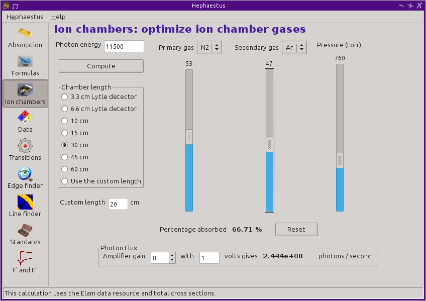
Fig. 13.5 The ion chambers tool.

13.4. Data

This tool is used to display a number of useful physical and chemical properties of the elements. Selecting an element from the periodic table will fill in a table with the data for that element.

Beneath the periodic table is a tabbed notebook. Each tab contains a different data table. The Elemental data tab contains a variety of general information. The Ionic radii tab contains the Shannon ionic radii. The Neutron data tab contains data on thermal neutron scattering lengths and cross sections for the major isotopes.

Fig. 13.6 The data tool.

General data

Swiped from https://edu.kde.org/kalzium/

Mossbauer data

List of Mossbauer active isotopes is from http://mossbauer.org, which used to be a site about Mossbauer spectroscopy but now seems to be a unmaintained science news site. Wikipedia has a nice periodic table of Mossbauer active elements and Darby Dyer keeps a lovely page about Mossbauer.

Ionic radii

• R. D. Shannon. Revised effective ionic radii and systematic studies of interatomic distances in halides and chalcogenides. Acta Crystallographica Section A, 32(5):751–767, Sep 1976. doi:10.1107/S0567739476001551.

Conversion of data to JSON at Electronic Table of Shannon Ionic Radii, J. David Van Horn, 2001, downloaded 10/13/2015.

Neutron data

• Varley F. Sears. Neutron scattering lengths and cross sections. Neutron News, 3(3):26–37, 1992. doi:10.1080/10448639208218770.

See also https://www.ncnr.nist.gov/resources/n-lengths/list.html Scattering lengths are in femtometers, cross sections are in barns (10E-24 cm), scattering lengths and cross sections in parenthesis are uncertainties, and for radioisotopes the half-life is given instead of the natural abundance.

13.5. Transitions

This tool displays a non-interactive chart explaining the transitions for each of the emission lines. The initial and final states for each named K and L transition is shown. The chart follows Figure 1.1 in the Center for X-Ray Optics X-Ray Data Booklet .

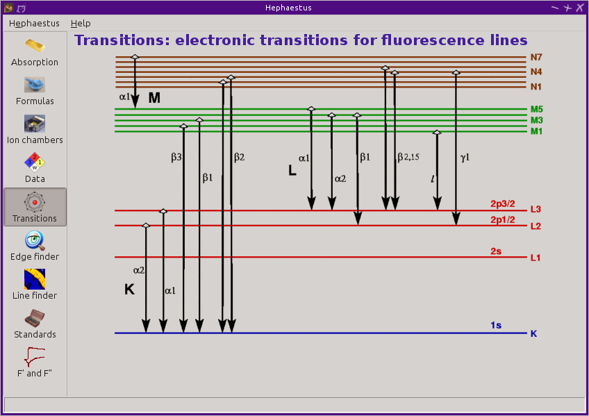
Fig. 13.7 The transitions tool.

13.6. Edge Finder

This tool displays a table, ordered by increasing edge energy, of all edge energies on the periodic table. The table also shows the edge energies in wavelength units and the core-hole lifetimes.

The purpose of this tool is to aid in identifying edges observed during measurements. To search the list, enter an energy in the text box on the right and click Search (or hit Return). The list will be recentered around that energy. Hopefully this will help you identify the mysterious feature in your measured data!

You can also search for edges at the second or third harmonic of the energy. This can be useful in the case of poor harmonic rejection in the incident beam and the excitation of a much higher energy edge.

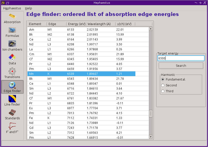
Fig. 13.8 The edge finder tool.

13.7. Line Finder

This tool displays a table, ordered by increasing emission energy, of all emission line energies on the periodic table. The table also shows the emission energies in wavelength units and the strength (or branching ratio) of each line relative to the other lines arising from the same absorption edge.

The purpose of this tool is to aid in identifying emission lines observed during measurements. To search the list, enter an energy in the text box on the right and click Search (or hit Return). The list will be recentered around that energy. Hopefully this will help you identify the mysterious line in your fluorescence data!

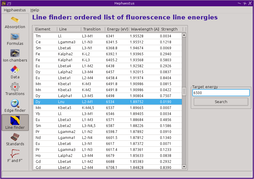
Fig. 13.9 The line finder tool.

13.8. Standards

Demeter is distributed with a small library of data on standard materials. These XANES spectra can be access via this tool. You will find that this library is quite tiny at this time. The hope is that a future effort in an XAS standards library will take off. When that happens, this will be HEPHAESTUS's interface to that effort.

Clicking on an element in the periodic table displays a list of all the standards in the library measured for that element. The disabled elements in the periodic table are ones for which the library has no entries.

The XANES data can be plotted as normalized μ(E) or as the derivative of μ(E). The data present have all been annotated so that interesting points are marked on the plots.

The Save button will prompt for a file name and save the μ(E) data to a file.

One point of this tool is to make obsolete the “Reference Spectra” printout from EXAFS Materials that is found at many beamlines. http://exafsmaterials.com/Ref_Spectra_0.4MB.pdf

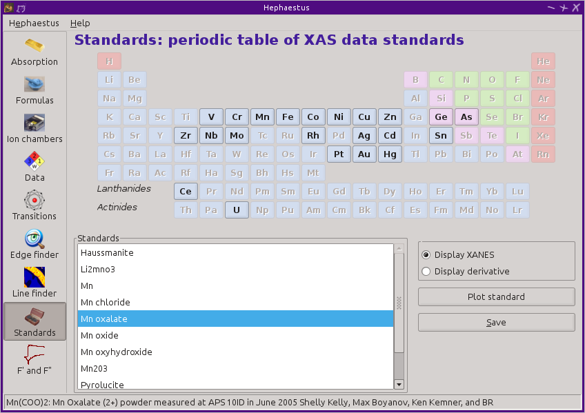
Fig. 13.10 The standards tool.

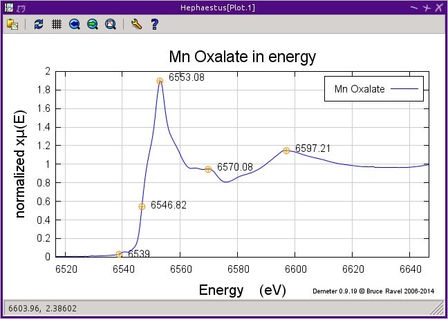
Fig. 13.11 An anotated standards plot for manganese oxalate.

The plotting range can be controlled using the ♦Hephaestus→standards_emin and ♦Hephaestus→standards_emax parameters.

13.9. F' and F"

This tool plots the complex anomalous scattering data from the Cromer-Liberman tables as a function of energy. The start and end energies for the plot are entered, as well as the energy grid spacing. When an element is selected from the periodic table, it's f' and f" values are plotted.

Anomalous scattering for elements can be plotted alone or over-plotted with other elements. You can also select to plot either f', f", or both.

The f' and f" data can be saved to a file.

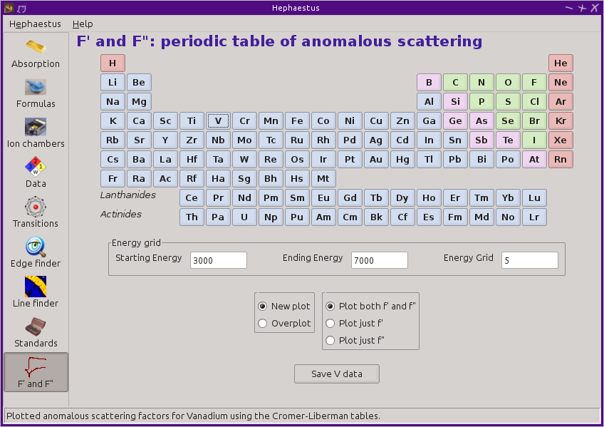
Fig. 13.12 The f' and f" tool.

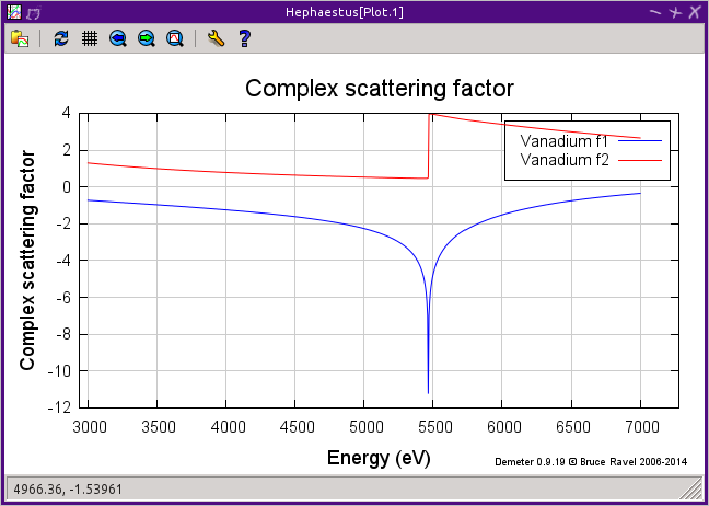
Fig. 13.13 An f' and f" plot for vanadium.

The plotting range can be controlled using the ♦Hephaestus→f1f2_emin and ♦Hephaestus→f1f2_emax parameters. The energy grid of the calculation is set using ♦Hephaestus→f1f2_grid.

13.10. Preferences

The behavior of HEPHAESTUS can be configured via the preferences tool. This uses the same preferences tool as ATHENA and ARTEMIS, although only those preference groups relevant to HEPHAESTUS and to plotting are presented.

Click on a group in the Parameters list to open a group. Click on a parameter to display it in the controls on the right. You will be given controls appropriate to each parameter's data type for setting the parameter value. The Your value and Demeter's value buttons can be used to restore a parameter's value. A description of the displayed parameter will be written in the large text box.

Parameters can be applied for the current session or applied and saved to your configuration file.

13.11. Credits

• The layout of HEPHAESTUS – with its button bar on the left side which changes the mode of the main part of the program – was inspired by the personal information management program I use on my KDE systems, Kontact. I found it effective so I swiped it for this program.
• The pictures used on the buttons were cropped from images I found using Google. The picture of the ion chamber is from the Advanced Designed Consulting web site. Their ion chambers are quite nice. The edge finder icon was swiped from the find.png icon in the kid's icon theme for KDE. The line finder icon is from a web page by the Alberta Synchrotron Institute and depicts a fluorescence map of some rock. The documentation icon was found under a Creative Commons license at http://battellemedia.com (but is no longer available at that site).
• The formulas utility owes much to Gerry Roe, who pointed out a bug, and Erik Gullikson, whose similar utility on the web set me straight.
• The ion chamber and edge finder utilities were inspired by the similar utilities in the data acquisition program by Lars Fuerenlid and Johnny Kirkland that was widely used at NSLS. Lars and Johnny seem to have a deeper love of pastel than do I.
• The electronic transitions chart was created from scratch but slavishly following Figure 1.1 in the Center for X-Ray Optics X-Ray Data Booklet .
• HEPHAESTUS makes use of several things from http://www.cpan.org
• And, of course, the users of my various software efforts deserve all the credit for kind praise and useful feedback over these many years.

The absorption data resources all have literature references.

The Elam tables

• W. T. Elam, B. D. Ravel, and J. R. Sieber. A new atomic database for X-ray spectroscopic calculations. Radiation Physics and Chemistry, 63:121–128, February 2002. doi:10.1016/S0969-806X(01)00227-4.

This is the source of data for the edge and line finders and for the filter plot.

The McMaster tables

• W. H. McMaster, N. Kerr Del Grande, J. H. Mallett, and J. H. Hubbell. Compilation of x-ray cross sections UCRL-50174, sections I, II revision 1, III, IV. Atomic Data and Nuclear Data Tables, 8:443–444, 1970. doi:10.1016/S0092-640X(70)80026-2.

These data were originally compiled in machine readable form by Pathikrit Bandyopadhyay.

The Henke tables

• B.L. Henke, E.M. Gullikson, and J.C. Davis. X-Ray Interactions: Photoabsorption, Scattering, Transmission, and Reflection at E = 50-30,000 eV, Z = 1-92. Atomic Data and Nuclear Data Tables, 54(2):181 – 342, 1993. doi:10.1006/adnd.1993.1013.

The data is available at http://henke.lbl.gov/optical_constants/

The Chantler tables

• C. T. Chantler. Theoretical Form Factor, Attenuation, and Scattering Tabulation for Z=1-92 from E=1–10 eV to E=0.4–1.0 MeV. Journal of Physical and Chemical Reference Data, 24(1):71–643, 1995. doi:10.1063/1.555974.

The data files can be found at http://physics.nist.gov/PhysRefData/FFast/html/form.html

The Cromer-Liberman tables

• S. Brennan and P. L. Cowan. A suite of programs for calculating x‐ray absorption, reflection, and diffraction performance for a variety of materials at arbitrary wavelengths. Review of Scientific Instruments, 63(1):850–853, 1992. doi:10.1063/1.1142625.

The Shaltout tables

• Abdallah Shaltout, Horst Ebel, and Robert Svagera. Update of photoelectric absorption coefficients in the tables of McMaster. X-Ray Spectrometry, 35(1):52–56, 2006. doi:10.1002/xrs.815.

13.12. Bugs and limitations

Every calculation at high energy is inaccurate in HEPHAESTUS. Xray::Absorption does not correctly handle the mass-energy absorption coefficients at high energy, although the ion chamber utility does attempt a (very) crude correction.

More types of information can be added to the chemical data utility. If there is something you would like to see, you should send the data in an easily readable format (i.e. plain text is lovely). Merely suggesting new data types is unlikely to have any effect. Supplying the data is highly likely to have an effect.

My wish list includes:

• auger/fluorescence branching ratios in the Data utility

• a tool for approximating the energy response of a flat mirror, like this or that

• providing the Berger/Hubble XCOM tables and FEFF's optical calculations as data resources.

  • MJ Berger, JH Hubbell, SM Seltzer, J Chang, JS Coursey, R Sukumar, DS Zucker, and K Olsen. XCOM: Photon cross sections database. NIST Standard reference database, 2013. URL: https://www.nist.gov/pml/xcom-photon-cross-sections-database.
  • M. P. Prange, J. J. Rehr, G. Rivas, J. J. Kas, and John W. Lawson. Real space calculation of optical constants from optical to x-ray frequencies. Phys. Rev. B, 80:155110, Oct 2009. doi:10.1103/PhysRevB.80.155110.

---

DEMETER is copyright © 2009-2016 Bruce Ravel – This document is copyright © 2016 Bruce Ravel

This document is licensed under The Creative Commons Attribution-ShareAlike License.

If DEMETER and this document are useful to you, please consider supporting The Creative Commons.