16.2. Silver/gold alloy
Topics demonstrated
- Multiple data set fitting
- using the characteristic value
In this example, a series of silver/gold alloys are co-refined using a simple model in which the first shell is a mixture of silver and gold backscatterers in the same proportion as the bulk. This example lends itself quite naturally to using the characteristic value of the Data object. It also demonstrates a direct manipulation of a Feff object without editing a feff.inp file.
1 2 3 4 5 6 7 8 9 10 11 12 13 14 15 16 17 18 19 20 21 22 23 24 25 26 27 28 29 30 31 32 33 34 35 36 37 38 39 40 41 42 43 44 45 46 47 48 49 50 51 52 53 54 55 56 57 58 59 60 61 62 63 64 65 66 67 68 69 70 71 72 73 74 75 76 77 78 79 80 81 82 83 84 85 86 87 88 89 90 91 92 93 94 95 96 97 98 99 100 101 102 103 104 105 106 107 108 109 110 111 112 113 | #!/usr/bin/perl
use Demeter qw(:ui=screen :plotwith=gnuplot);
print "Multiple data set fit to several AgAu samples using Demeter $Demeter::VERSION\n";
### -------- import five sets of Ag and Ag/Au data from an Athena project file
my $prj = Demeter::Data::Prj->new(file => 'AgAu_merged.prj');
$prj -> set_mode(screen=>0, backend=>1);
my @common = (fft_kmin => 2, fft_kmax => 11,
bft_rmax => 3.2, bft_rmin => 1.8,
fit_k1 => 1, fit_k2 => 0, fit_k3 => 1,);
my $data_100 = $prj->record(1);
$data_100 -> set(@common, cv => 1, name => 'pure silver');
my $data_80 = $prj->record(3);
$data_80 -> set(@common, cv => 0.8, name => '80% silver');
my $data_60 = $prj->record(5);
$data_60 -> set(@common, cv => 0.6, name => '60% silver');
my $data_50 = $prj->record(6);
$data_50 -> set(@common, cv => 0.5, name => '50% silver');
my $data_40 = $prj->record(7);
$data_40 -> set(@common, cv => 0.4, name => '40% silver');
## -------- make GDS objects for an isotropic expansion, correlated
## Debye, mixed first shell fit to silver and silver/gold
my @gdsobjects = ($data_100 -> simpleGDS("guess amp = 1"),
$data_100 -> simpleGDS("guess enot = 0"),
$data_100 -> simpleGDS("guess dr_ag = 0"),
$data_100 -> simpleGDS("guess ss_ag = 0.003"),
$data_100 -> simpleGDS("guess dr_au = 0"),
$data_100 -> simpleGDS("guess ss_au = 0.003"),
## Determine Ag::Au ratios with an lguess
## $data_100 -> simpleGDS("lguess frac = 0.6"),
);
## -------- import Ag crystal data and generate a feff.inp file
my $atoms = Demeter::Atoms->new(file => "Ag.inp");
open(my $FEFF, '>feff.inp');
print $FEFF $atoms->Write("feff6");
close $FEFF;
## -------- run Feff on pure silver
my $agfeff = Demeter::Feff -> new(file => "feff.inp");
$agfeff -> set(workspace=>"feff/", screen=>0,);
$agfeff -> make_workspace;
$agfeff -> run;
## -------- make a path object from the 1st shell of pure silver, use
## this for the pure silver data
my @paths = ();
$paths[0] = Demeter::Path -> new();
$paths[0]->set(data => $data_100,
parent => $agfeff,
sp => $agfeff->pathlist->[0],
name => 'silver',
n => 12,
s02 => 'amp',
e0 => 'enot',
delr => 'dr_ag',
sigma2 => 'ss_ag',
);
## -------- clone the Ag Feff calculation, add Au to the potentials
## list, make an Au scatterer out of the first site after the
## absorber
my $aufeff = $agfeff->Clone;
$aufeff -> set(workspace=>"feffau/", screen=>0,);
$aufeff -> make_workspace;
$aufeff -> push_potentials([2, 79, 'Au']); ## add Au to the end of the potentials list
my @sites = @{ $aufeff->sites }; ## make the first atom after the
my @neighbor = @{ $sites[1] }; ## absorber in the sites list an Au
@neighbor[3,4] = (2,'Au'); ## (this could be easier...)
$sites[1] = \@neighbor;
$aufeff -> sites(\@sites);
$aufeff -> run; ## and continue
## -------- clone the Path object several times, taking care to
## correctly map paths to data sets
my %map = (2=>$data_80, 4=>$data_60, 6=>$data_50, 8=>$data_40);
my %percentage = (2=>'80', 4=>'60', 6=>'50', 8=>'40');
foreach my $i (2,4,6,8) { # clone silver paths
my $j = $i-1;
$paths[$j] = $paths[0]->Clone(data => $map{$i},
#s02 => "amp*frac", # lguess
s02 => "amp*[cv]", # char. value
);
};
foreach my $i (2,4,6,8) { # clone gold paths
my $j = $i-1;
$paths[$i] = $paths[$j]->Clone(parent => $aufeff,
sp => $aufeff->find_path(tag=>['Au']),
name => "gold",
n => 12,
#s02 => "amp*(1-frac)", # lguess
s02 => "amp*(1-[cv])", # char. value
delr => "dr_au",
sigma2 => "ss_au",
);
};
## -------- make a Fit object, which is just a collection of GDS, Data, and Path objects
my $fitobject = Demeter::Fit -> new;
$fitobject->set(gds => \@gdsobjects,
data => [$data_100, $data_80, $data_60, $data_50, $data_40],
paths => \@paths
);
## -------- do the fit
$fitobject -> fit;
$fitobject -> interview;
|
An ATHENA project file is imported at line 6. At lines 11
through 24, five of the data sets from the project file are imported
into Data objects. Each one has its name cv attributes set
appropriately. The cv is set to the bulk fradction of silver in
the sample.
A set of guess parameters is defined at lines 28-33 for a simple fitting model that includes overall amplitude and E0 parameters along with ΔR and σ2 parameters for each type of scatterer.
At line 39-42 an atoms.inp is imported and a temporary
feff.inp is written. This feff.inp is imported,
forming a Feff object at line 45. Note that the run method at
line 48 is a wrapper around the potph and pathfinder methods.
The first path from this calculation, the one corresponding to the 12
silver atoms in the first coordination shell, is made into a Path
object at lines 53-63. Note the idiomatic dereferencing of the first
ScatteringPath object from the FEFF calculation at
line 56. Note that this Path object points at the Data object for the
pure silver data.
The FEFF calculation for the contribution from the Au scatterer is obtained at lines 68-77. Here's how it works. First, the Feff object from the pure silver calculation is cloned at line 68 and a separate workspace is established at lines 69 and 70. At line 71, a new potential type is pushed onto the list of potentials of the cloned Feff object. At lines 72-76, an atom from the first coordination shell is switched from silver to gold. This modified sites list is then pushed back into the object.
The manipulations at lines 68-77 represent both a weakness and a great strength of DEMETER's interactions with FEFF. On one hand, DEMETER currently lacks more graceful tools for making these manipulations. On the other hand, this example demonstrates the extent to which a FEFF calculation can be controlled algorithmically. Thus complex modeling chores can be programed directly rather than prepared on disk beforehand.
At lines 81-101, paths are set up for the four alloy samples. First, at
83-89, the silver path is cloned and assigned to each alloy Data object.
Note that the characteristic value is used to get the
amplitude term set correctly for each alloy Data object. In this case,
the cv is set to the amount of silver in each sample. When the
[cv] token is resolved, each silver path will have its amplitude set
properly.
At lines 90-101, more paths are cloned, then modified to use the
ScatteringPath object which corresponds to the gold scatterer from the
second FEFF calculation. Again, care is taken to make sure
that the correct Path object, with the correct cv value, is
associated with the correct Data object. Note the use of the
find_path method at line 93. This identifies the ScatteringPath
object using a semantic path description.
This simplifies the chore of finding the correct ScatteringPath
without needing to keep track of the order of scattering paths in the
FEFF calculation.
Finally, the Fit object is created and the fit is run. Finally, the
interview method is called so the fit can be examined interactively
from a command line script.
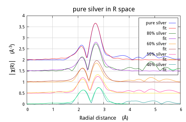
Fig. 16.3 Fit to the ensemble of Ag/Au alloy data.
The lines below replaced the interview method to produce this
plot of the result of the fit:
$fitobject -> po -> set(plot_fit =>  1,
                        r_pl     => 'm',
                        kweight  =>  2);
$data_100  -> y_offset(2.0);
$data_100  -> plot('r');

$data_80   -> y_offset(1.5);
$data_80   -> plot('r');

$data_60   -> y_offset(1.0);
$data_60   -> plot('r');

$data_50   -> y_offset(0.5);
$data_50   -> plot('r');

$data_40   -> y_offset(0.0);
$data_40   -> plot('r');
$data_40   -> pause;
As a final note, the fit presented here assumes that the mixture of silver and gold in the first coordination shell is of the same ratio as the nominal bulk mixing ratios. This assumption can be easily relaxed. By uncommenting lines 35, 86, and 96 and commenting out line 87 and 97, the fixed mixing ratios are turned into a guess parameter for each data set using a local guess parameter. In this way, the lguess is expanded into 5 guess parameters, one for each data set. Try it!
DEMETER is copyright © 2009-2016 Bruce Ravel – This document is copyright © 2016 Bruce Ravel
This document is licensed under The Creative Commons Attribution-ShareAlike License.
If DEMETER and this document are useful to you, please consider supporting The Creative Commons.