16.4. Histogram

Topics demonstrated:

• Fitting using an arbitrary distribution of atoms

In a simple fitting model, such as the fit to copper metal, we assume that the neighboring atoms are Gaussian distributed and that all disorder about the near-neighbor scattering distance can be described by the application of the σ² term in the EXAFS equation. Often, this is quite enough. For well-ordered materials, it is probably even true. For small levels of structural disorder, the additional disorder thus introduced can often be approximated by having a larger σ² value or by introducing a small number of additional scattering paths at slightly different distances.

Some systems, however, are not well described by a Gaussian distribution. When the structural disorder is sufficeintly large, a simple Gaussian is inadequate to describe the distribution. In the EXAFS literature, higher cumulants are often used in this situation. But even this approach is limited in that, in practice, one can only measure small third and fourth cumulants (i.e. a skew and a kurtosis of the distribution) with any precision.

In this example, I explain one method for incorporating the results of a molecular dynamics simulation into an EXAFS analysis. The system is a very small metallic gold nanoparticle. The very large ratio of surface area to volume introduces substantial distortions to the local structure of the particle. These local structural distortions are seen in the MD simulations. From these MD simulations, we have files containing the local structure in the form of a histogram. These files contain some measure of the probability of finding a neighboring atom on a grid of radial distances. It looks something like this:

0.000  0.000000E+00
.
  .
    .
2.636  2.818836E-01
2.642  3.801608E+00
2.649  1.245984E+01
2.656  1.017059E+00
2.662  1.660477E-01
2.668  6.903760E-02
2.675  5.119136E-02
2.681  6.556027E-02
2.688  1.158219E-01
.
  .
    . and so on out to about 6.5 A

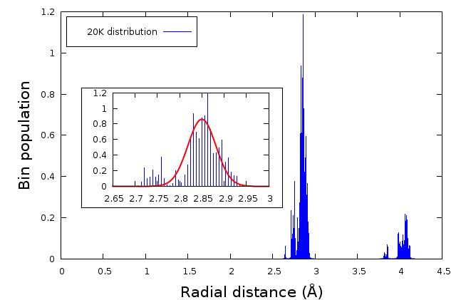
Fig. 16.8 Here is a plot of one calculated pair distribution function for these metallic gold nanoparticles. The main plot shows the distribution of atoms in the first two coordination shells. The bin populations have been normalized such that the first coordination shell contains 12 atoms. The inset shows a blow-up of the first coordination shell along with a Gaussian fitted to that distribution.

From the inset to this figure, we see that a Gaussian is not a very good representation of this distribution. It does an ok job of representing the bulk of the coordination shell, but it completely fails to represent the smaller population of shorter Au-Au distances which, presumably, result from truncation effects at the relatively large surface.

The approach the DEMETER offers is to compute an SSPath at each bin of the histogram. The at each bin is set to the population of that bin. Each bin should get the same E₀ parameter. If the histogram accurately represents all soruces of disorder – both structural and thermal, something that is certainly possible in an MD simulation – then no σ² or ΔR parameters would be needed. Of course, they could be introduced to account for any shortcomings of the MD simulation compared to the measured data.

 #!/usr/bin/perl
 use Demeter qw(:plotwith=gnuplot :ui=screen);

 ## -------- Import the results of a Feff calculation on bulk Au
 my $feff = Demeter::Feff->new(yaml=>'Au_feff.yaml');
 $feff->set(workspace=>"./", screen=>0,);
 my @list_of_paths = @{ $feff->pathlist };

 ## -------- Import some data
 my $data  = Demeter::Data::Prj->new(file=>'Aunano.prj') -> record(5);
 $data -> set(fft_kmin => 3,      fft_kmax => 13,
              bft_rmin => 1.992,  bft_rmax => 3.399,
              fit_k1   => 1,      fit_k2   => 1,     fit_k3=>1, );

 ## -------- Import the first scattering path object and use it
 ##          to populate a histogram defined by an external file.
 ##          Also define a VPath containing the entire first
 ##          shell of the histogram.
 my $firstshell = $list_of_paths[1];

 my ($rx, $ry) = $firstshell->histogram_from_file('histogram_file', 1, 2, 2.5, 3.1);
 my $common = [data=>$data, sigma2 => 'sigsqr', e0 => 'enot', delr => 'alpha*reff'];

 my $paths = $firstshell -> make_histogram($rx, $ry, 'amp', q{}, $common);
 my $vpath = Demeter::VPath->new(name=>'histo');
 $vpath->include(@$paths);

 ## -------- Some parameters
 my @gds = (
            Demeter::GDS->new(gds=>'guess', name=>'amp',    mathexp=>6),
            Demeter::GDS->new(gds=>'guess', name=>'enot',   mathexp=>0),
            Demeter::GDS->new(gds=>'set',   name=>'alpha',  mathexp=>0),
            Demeter::GDS->new(gds=>'set',   name=>'sigsqr', mathexp=>0.0),
           );
 $data->po->kweight(2);

 ## -------- Do the fit
 my $fit = Demeter::Fit->new(gds=>\@gds, data=>[$data], paths=>$paths);
 $fit->fit;
 $fit->interview;

At line 5-7 a FEFF calculation on gold metal is imported. This calculation was made and frozen to the Au_feff.yaml file ahead of time. (See here for details.) We will only be using the first ScatteringPath object from the path list. That is the contribution from the first coordination shell and will be used as the basis for the historgram.

At lines 10-13, data are imported from an ATHENA project file. At line 19, a reference to the ScatteringPath object for the first coordination shell is stored in the $firstshell variable.

All the interesting stuff in this example happens between lines 21 and 26. First, the locations and populations of the histogram are read from a column data file at line 21. The histogram_from_file method (which is a method of the ScatteringPath object) takes 5 arguments – the file name, the column numbers of the bin positions and bin populations, and the range in R-space. Bins in the histogram that lie outside the R-range will not be considered. An example of a histogram file is shown above. This method returns two scalars which are references to the arrays containing the bin positions and populations, i.e. the x and y arrays of the histogram. To examine these arrays, you would have to dereference these scalars:

my @bin_positions = @$rx

At line 22, an anonymous array of path parameters values is created. These values will be used for every Path object created by histogram generating method. Note that I am using this anonymous array to pass various attributes to the Path objects in the histogram. Passing these in this way is just a convenience – they could be set after the fact instead.

At line 24, the set of Path objects representing the contribution from each bin of the histogram is actually generated using the make_histogram method (also a method of the ScatteringPath object). This method takes 4 arguments. The first two are the array references returned by the histogram_from_file method. The last argument is the array reference created at line 22. Each item in the array will be passed on to each of the Path objects that gets generated.

The third argument of the make_histogram method is very important! It is the name of the amplitude parameter that will be varied in the fit. Each path parameter for every generated path will be given a math expression that is this amplitude parameter multiplied by the unit-normalized bin population. Since the histogram is unit normalized, this parameter represents the total coordination number multiplied by the S²₀ value.

At lines 25 and 26, a VPath object is created to hold the contribution from the entire histogram. This is particularly handy as a visualization tool if the histogram is just one part of the fit.

Finally a set of GDS object are defined and the fit is run. Note that an overall σ² parameter has been defined but set to 0. An isotropic expansion parameter has also been defined but set to zero.

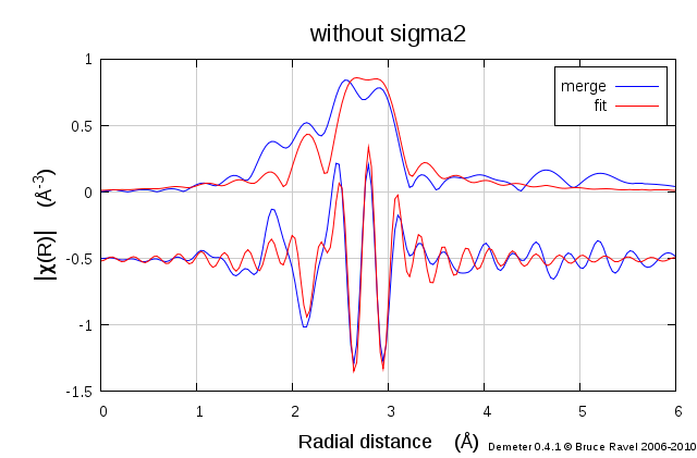
Fig. 16.9 Here is the result of the fit varying on S²₀ and E₀. The σ² parameter has been fixed to 0. This fit isn't great, but it is not horrible either. It seems safe to say that the distribution used here is not an adequate representation of the complete structural and thermal disorder in this particular system.

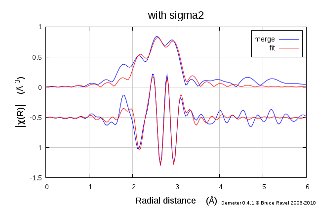
Fig. 16.10 In this fit, the σ² parameter has been set to be a guess parameter. It returns a non-zero value and substantially improves the fit. Whatever disorder was not considered in the input configuration was accounted for to some extent by the addition of this parameter.

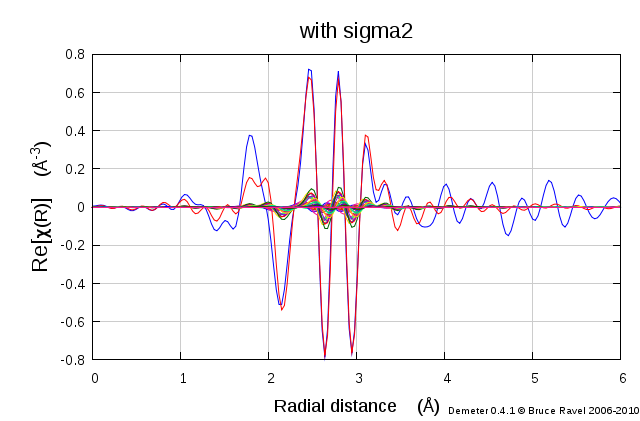
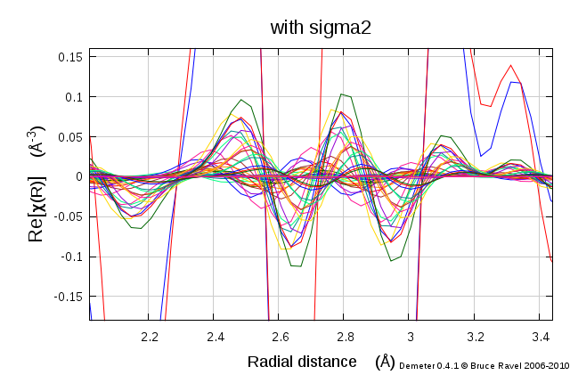
To fully understand how the histogram concept works, it is useful to see the contribution from each bin in the histogram along with the data and the fit.

Fig. 16.11 The fit with σ² floated showing the contributions from each bin of the histogram. Each individual bin contributes only a small amount of the spectral weight, but together they add up to the result.

Fig. 16.12 Zooming in on the contributions from each bin. Note the complicated phase relationship of these paths which contributes to the overall fit.

---

DEMETER is copyright © 2009-2016 Bruce Ravel – This document is copyright © 2016 Bruce Ravel

This document is licensed under The Creative Commons Attribution-ShareAlike License.

If DEMETER and this document are useful to you, please consider supporting The Creative Commons.