4.1. Normalization

Normalization is the process of regularizing your data with respect to variations in sample preparation, sample thickness, absorber concentration, detector and amplifier settings, and any other aspects of the measurement. Normalized data can be directly compared, regardless of the details of the experiment. Normalization of your data is essential for comparison to theory. The scale of the μ(E) and χ(k) spectra computed by FEFF is chosen for comparison to normalized data.

The relationship between μ(E) and χ(k) is:

μ(E) = μ₀(E) * (1 + χ(E))

which means that

χ(E) = (μ(E) - μ₀(E)) / μ₀(E)

The approximation of μ₀(E) in an experimental spectrum is a topic that will be discussed shortly.

This equation is not, in fact, the equation that is commonly used to extract χ(k) from the measured spectrum. The reason that equation is problematic is the factor of μ₀(E) in the denominator. In practice, one cannot trust the μ₀(E) to be sufficiently well behaved that it can be used as a multiplicative factor. An example is shown below.

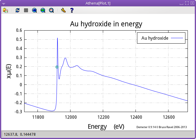
Fig. 4.1 μ(E) data for gold hydroxide, which crosses the zero axis in the EXAFS region.

In the case of the gold spectrum, the detector setting were such that the spectrum crosses the zero-axis. Dividing these spectra by μ₀(E) would be a disaster as the division would invert the phase of the extracted χ(k) data at the point of the zero-crossing.

To address this problem, we typically avoid functional normalization and instead perform an edge step normalization. The formula is

χ(E) = (μ(E) - μ₀ (E)) / μ₀(E₀)

The difference is the term in the denominator. μ₀(E₀) is the value of the background function evaluated at the edge energy. This addresses the problem of a poorly behaved μ₀ (E) function, but introduces another issue. Because the true μ₀ (E) function should have some energy dependence, normalizing by μ₀(E₀) introduces an attenuation into χ(k) that is roughly linear in energy. An attenuation that is linear in energy is quadratic in wavenumber. Consequently, the edge step normalization introduces an artificial σ² term to the χ(k) data that adds to whatever thermal and static σ² may exist in the data.

This artificial σ² term is typically quite small and represents a much less severe problem than a misbehaving functional normalization.

4.1.1. The normalization algorithm

The normalization of a spectrum is controlled by the value of the «e0», «pre-edge range», and «normalization range» parameters. These parameters are highlighted in this screenshot.

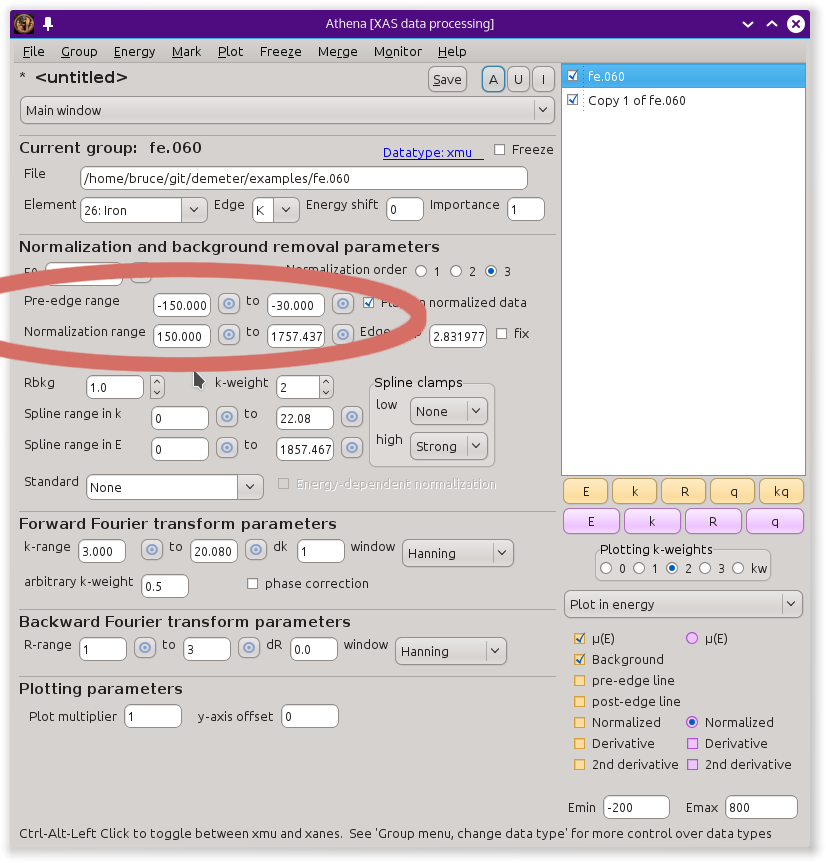
Fig. 4.2 Selecting the normalization parameters in ATHENA.

The «pre-edge range» and «normalization range» parameters define two regions of the data – one before the edge and one after the edge. A line is regressed to the data in the «pre-edge range» and a polynomial is regressed to the data in the «normalization range». By default, a three-term (quadratic) polynomial is used as the post-edge line, but its order can be controlled using the «normalization order» parameter. Note that all of the data in the «pre-edge range» and in the «normalization range» are used in the regressions, thus the regressions are relatively insensitive to the exact value of boundaries of those data ranges.

The criteria for good pre- and post-edge lines are a bit subjective. It is very easy to see that the parameters are well chosen for these copper foil data. Both lines on the left side of this figure obviously pass through the middle of the data in their respective ranges.

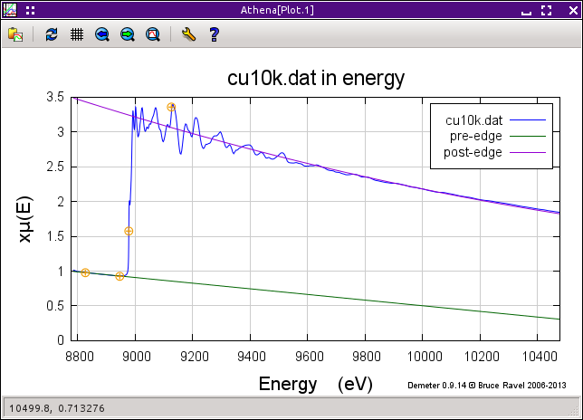
Fig. 4.3 Cu foil μ(E) with pre and post lines.

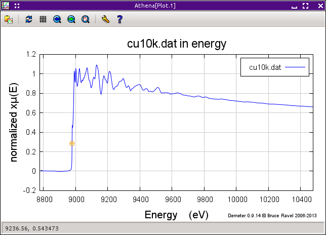
Fig. 4.4 Normalized μ(E) data for a copper foil.

Data can be plotted with the pre-edge and normalization lines using controls in the energy plot tabs. It is a very good idea to visually inspect the pre-edge and normalization lines for at least some of your data to verify that your choice of normalization parameters is reasonable.

When plotting the pre- and post-edge lines, the positions of the «pre-edge range», and «normalization range» parameters are shown by the little orange markers. (The upper bound of the «normalization range» is off screen in the plot above of the copper foil.)

The normalization constant, μ₀(E₀) is evaluated by extrapolating the pre- and post-edge lines to «e0» and subtracting the e0-crossing of the pre-edge line from the e0-crossing of the post-edge line. This difference is the value of the «edge step» parameter.

The pre-edge line is extrapolated to all energies in the measurement range of the data and subtracted from μ(E). This has the effect of putting the pre-edge portion of the data on the y=0 axis. The pre-edge subtracted data are then divided by μ₀(E₀). The result is shown on the right side of the figure above.

New in version 0.9.18,: an option was added to the context menu attached to the «edge step» label for approximating the error bar on the edge step.

4.1.2. The flattening algorithm

For display of XANES data and certain kinds of analysis of μ(E) spectra, ATHENA provides an additional bit of sugar. By default, the flattened spectrum is plotted in energy rather than the normalized spectrum. In the following plot, flattened data are shown along with a copy of the data that has the flattening turned off.

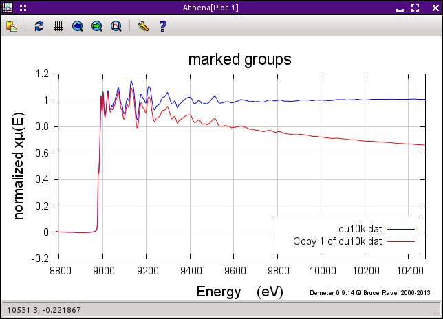
Fig. 4.5 Comparing normalized (red) and flattened (blue) data using a Cu foil.

To display the flattened data, the difference in slope and quadrature between the pre- and post-edge lines is subtracted from the data, but only after «e0». This has the effect of pushing the oscillatory part of the data up to the y=1 line. The flattened μ(E) data thus go from 0 to 1. Note that this is for display and has no impact whatsoever on the extraction of χ(k) from the μ(E) spectrum.

This is a nice way of displaying XANES data as it removes many differences in the shape of the post-edge region from the data. Computing difference spectra or self absorption corrections, performing linear combination fitting or peak fitting, and many other chores often benefit from using flattened data rather than simply normalized data.

This idea was swiped from SixPACK.

4.1.3. Getting the post-edge right

It is important to always take care selecting the post-edge range. Mistakes made in selecting the «normalization range» parameters can have a profound impact on the extracted χ(k) data. Shown below is an extreme case of a poor choice of «normalization range» parameters. In this case, the upper bound was chosen to be on the high energy side of a subsequent edge in the spectrum. The resulting «edge step» is very wrong and the flattened data are highly distorted.

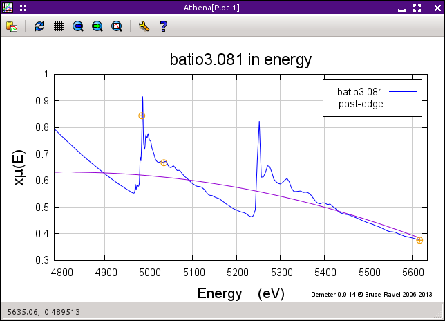
Fig. 4.6 The post-edge line is chosen very poorly for this BaTiO₃ spectrum. The upper end of the normalization range is on the other side of the Ba L_III edge.

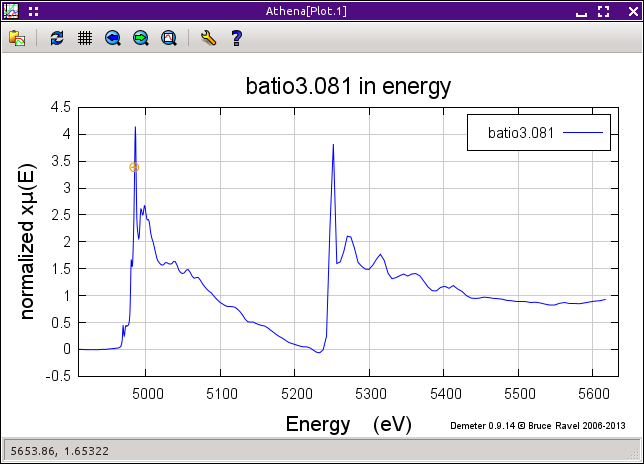
Fig. 4.7 The poor choice of normalization range for BaTiO₃ results in very poorly normalized Ti K edge data.

The previous example is obviously an extreme case, but it illustrates the need to examine the normalization parameters as you process your data. In many cases, subtle mistakes in the choice of normalization parameters can have an impact on how the XANES data are interpreted and in how the χ(k) data are normalized.

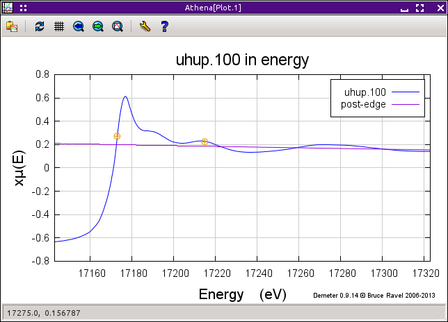
Fig. 4.8 One choice of «norm1».

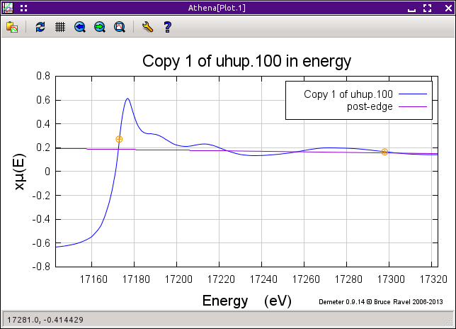
Fig. 4.9 Another choice of «norm1».

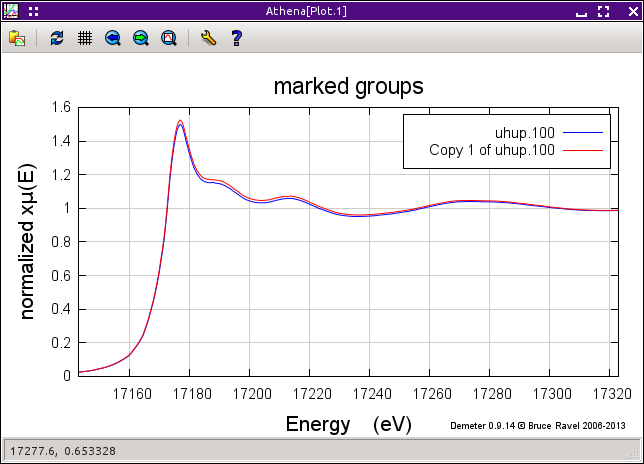
Fig. 4.10 Example of a subtle effect in how the post-edge line is chosen in a hydrated uranyl species. This compared the flattened XANES data for different choices of post-edge line in a hydrated uranyl species.

In this example, the different choice for the lower bound of the normalization range (42 eV in one case, 125 eV in the other) has an impact on the flattening of these uranium edge data data, which in turn may have in impact in the evaluation of average valence in the system. The small difference in the «edge step» will also slightly attenuate χ(k).

4.1.4. Getting the pre-edge right

The choice of the «pre-edge range» parameters is similarly important and also requires visual inspection. A poor choice can result in an incorrect value of the «edge step» and in distortions to the flattened data. In the following spectrum, we see the presence of a small yttrium K-edge at 17038 eV which distorts the pre-edge for a uranium L_III-edge spectrum at 17166 eV as shown in the figure below. In this case the «pre-edge range» should be chosen to be entirely above the yttrium K-edge energy.

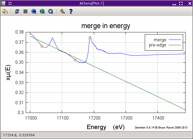
Fig. 4.11 A sediment sample with both uranium and yttrium.

4.1.5. Measuring and normalizing XANES data

If time and the demands of the experiment permit, it is always a good idea to measure significant amounts of the pre- and post-edge regions. About 150 volts in the pre-edge and at least 300 volts in the post-edge is a good rule of thumb. With shorter regions, it may be difficult to find normalization boundaries that provide good normalization lines. Without a good normalization, it can be difficult to compare a XANES measurement quantitatively with other measurements.

Reducing the «normalization order» might help in the case of limited post-edge range. When measuring XANES spectra in a step scan, it is often a good idea to add several widely spaced steps to the end of a scan to extend the «normalization range» without adding excessive time to scan.

---

DEMETER is copyright © 2009-2016 Bruce Ravel – This document is copyright © 2016 Bruce Ravel

This document is licensed under The Creative Commons Attribution-ShareAlike License.

If DEMETER and this document are useful to you, please consider supporting The Creative Commons.