9.9. Self-absorption approximations
 The statement that μ(E) measured in fluorescence
is the ratio of the signals on the fluorescence and incident ion
chambers is only true in the limit of very thin samples or very dilute
samples. For thick, concentrated samples, the depth into which the
incident beam can penetrate changes as fine structure of μ(E)
changes. As the oscillatory part wiggles up, the penetration depth
diminishes. As it wiggles down, the depth increases. This serves to
attenuate the oscillatory structure.
The statement that μ(E) measured in fluorescence
is the ratio of the signals on the fluorescence and incident ion
chambers is only true in the limit of very thin samples or very dilute
samples. For thick, concentrated samples, the depth into which the
incident beam can penetrate changes as fine structure of μ(E)
changes. As the oscillatory part wiggles up, the penetration depth
diminishes. As it wiggles down, the depth increases. This serves to
attenuate the oscillatory structure.
Attention
The term “self-absortion” is sort of a misnomer and is confusing when compared to what the term means in other areas. For example, in X-ray fluorescence, “self-absorption” actually means the attenuation of fluorescence generated within a sample as it travels out of the sample, which is different from the effect discussed here. The term “self-absorption” was first used in the Troger reference to describe an effect first described in the much earlier paper by Goulon, et al. Many in the XAS community prefer the term “over-absorption” or Goulon's phrase “attenuation factor”.
- L. Tröger, D. Arvanitis, K. Baberschke, H. Michaelis, U. Grimm, and E. Zschech. Full correction of the self-absorption in soft-fluorescence extended x-ray-absorption fine structure. Phys. Rev. B, 46:3283–3289, Aug 1992. doi:10.1103/PhysRevB.46.3283.
- Goulon, J., Goulon-Ginet, C., Cortes, R., and Dubois, J.M. On experimental attenuation factors of the amplitude of the EXAFS oscillations in absorption, reflectivity and luminescence measurements. J. Phys. France, 43(3):539–548, 1982. doi:10.1051/jphys:01982004303053900.
Ideally, all your samples that must be measured in fluorescence should be either sufficiently thin or sufficiently dilute that your data is unaffected by this self-absorption effect. Sometimes, the constraints of the sample are such that self-absorption cannot be avoided. In that case, you need to figure out what to do at the level of the data analysis to find the correct answer in the face of this problem. One solution is presented here.
The self-absorption correction tool offers four different algorithms to approximate the effect of self-absorption using tables of x-ray absorption coefficients. One of them works on XANES data, while all four can be used to correct EXAFS data. One of the algorithms works well for samples that are not in the infinitely thick limit. These various algorithms are taken from the available literature and are offered to allow you to compare.
The examples I show here are particularly well suited to this sort of correction. In both cases, we have a way to evaluate the success of the correction. In general, it can be difficult to guarantee the success of the correction, particularly if the entire composition of the sample is not well known. That means that, in practice, this sort of correction may not be useful or reliable.
It is also important to understand that the self-absorption effect only effects the amplitude of your EXAFS data, not the phase. Thus even if you are unable to properly correct, you can still analyze your EXAFS data for bond lengths.
Here is my presentation on self-absorption corrections. There I discuss the applicability of this tool in more detail. You will find that, in general, the self-absorption tool is very hard to apply to real data. There is quite a bit of useful information on this topic at XAFS.org.
9.9.1. Correcting XANES data
The self-absorption tool below allows you to choose between the four algorithms and to provide the parameters of the correction.
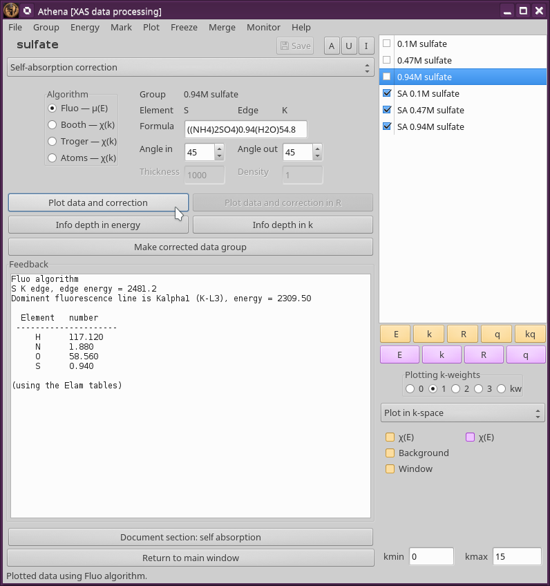
Fig. 9.24 The self-absorption tool.
In this example of correcting XANES data, ammonium sulfate was dissolved in water at three different molarities: 0.1, 0.47, and 0.94. The correction algorithm requires a complete description of the sample, so we need to determine the ratio of water to ammonium sulfate.
1 amu = 1.6605 x 10^-27 kg

1 mole = 6.0221 x 10^23 particles

1 water molecule is 18 amu = 2.988 x 10^-26 kg

1 mole of water is .01800 kg

1 liter of water = 1 kg water, so 1 liter is 55.5555 moles
Adjusted for the density change upon adding the solute, there are about 54.8 moles of water in the solution
So the formulas for these three molar solution are ((NH4)2SO4)0.10(H2O)54.8, ((NH4)2SO4)0.47(H2O)54.8, and ((NH4)2SO4)0.94(H2O)54.8.
The uncorrected and corrected data for the 0.94M sample are shown here on the right. The three uncorrected spectra are shown on the left and the corrected spectra are shown on the bottom.
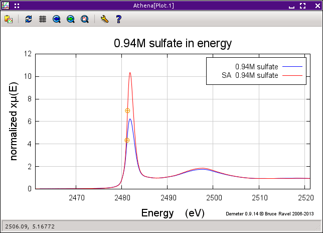
Fig. 9.25 This is the 0.94M data corrected by this algorithm.
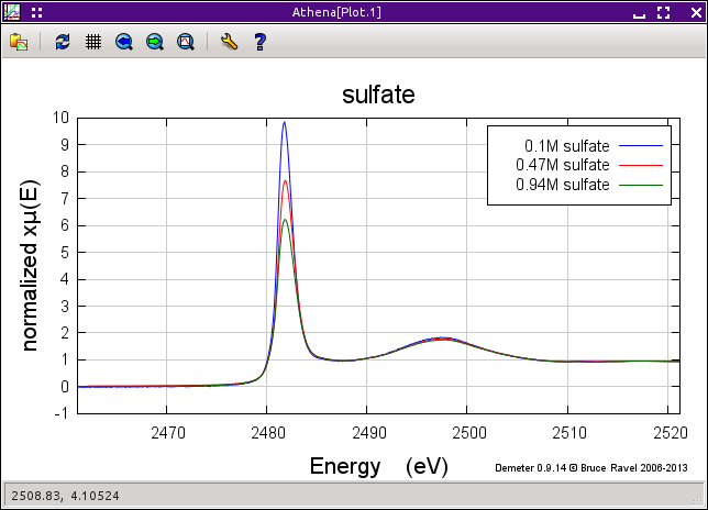
Fig. 9.26 Here is the raw data for the three samples. You can see the effect of self-absorption growing for the more concentrated samples.
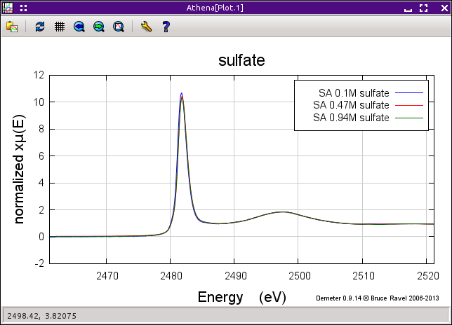
Fig. 9.27 The corrected data. Not bad, eh?
Thanks to Dani Haskel and Zhang Ghong for these data.
9.9.2. Correcting EXAFS data
Of the four algorithms, only the Booth algorithm as shown in this figure is suitable for samples of finite thickness. The other three all assume that samples are infinitely thick.
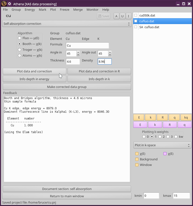
Fig. 9.28 The self-absorption tool with copper data for correction using the Booth algorithm.
After selecting an algorithm, you can use the other controls to enter the incident and outgoing angles in degree, the thickness of the sample in microns, and the density as specific gravity. All algorithms require that you specify the formula of the sample with stoichiometries in atomic percent.
These two data groups were measured from the same thin copper foil, one in transmission and the other in fluorescence. These data were provided by Corwin Booth and are the data from the paper where he and Bud Bridges presented their algorithm (citation below).
Since this is a thin film, only the Booth algorithm is appropriate. (Although you might want to compare it to the other algorithms, if only to see how the others overestimate the size of the correction due to the fact that they do not consider film thickness.)
The formula for copper is Cu and Corwin reports that the thickness of the sample is 4.6, the incident was 49 degrees and the outgoing angle was 41 degrees. Enter these values and plot the correction. Save the corrected data group and compare it to the transmission data, as shown in the plot below.
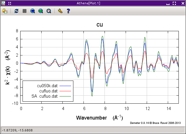
Fig. 9.29 It works pretty well. The green trace is the corrected fluorescence spectrum, which compares well to the transmission data, albeit a little too big.
There are several things that can effect the comparison of the corrected fluorescence data and the transmission data. These include how the two data sets were normalized, the incident and outgoing angles, and the thickness. Try changing all those things to see how they effect the correction.
New in version 0.9.20: The Booth algorithm was updated and corrected. It now requires that the density of the material be provided. There is a box for the density next to the thickness box. The density box becomes enabled (not grayed out) when the Booth algorithm is selected.
9.9.3. Information depth
For any sample, you can plot the information depth as a function of wavenumber. This quantity was defined by Troger et al. (citation below) and represents the depth into the sample probed by the incident beam for a given sample geometry as a function of energy. In that depth, 68 percent of the incident photons are absorbed and 68 percent of the fluorescence photons are generated. The information depth provides a useful metric for whether a film sample can be considered “thick” in a particular experiment.
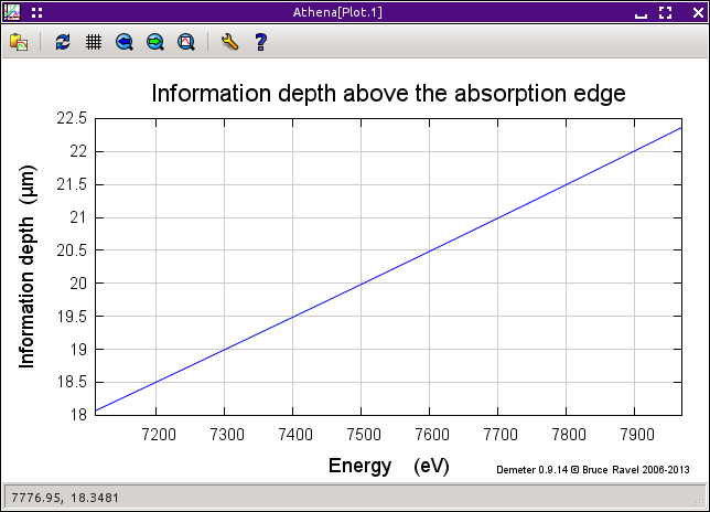
Fig. 9.30 The information depth for an iron/gallium alloy, plotted in energy.
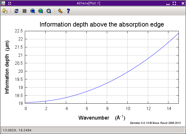
Fig. 9.31 The same plot, but in wavenumber.
9.9.4. Algorithm references
- Fluo algorithm
- The program documentation for Fluo can be found at Dani's web site and includes the mathematical derivation: http://www.aps.anl.gov/ haskel/fluo.html
- Booth Algorithm
- C H Booth and F Bridges. Improved self-absorption correction for fluorescence measurements of extended x-ray absorption fine-structure. Physica Scripta, 2005(T115):202, 2005. doi:10.1238/Physica.Topical.115a00202.
See also Corwin's web site: http://lise.lbl.gov/RSXAP/
- Troger Algorithm
- L. Tröger, D. Arvanitis, K. Baberschke, H. Michaelis, U. Grimm, and E. Zschech. Full correction of the self-absorption in soft-fluorescence extended x-ray-absorption fine structure. Phys. Rev. B, 46:3283–3289, Aug 1992. doi:10.1103/PhysRevB.46.3283.
- Pfalzer Algorithm
Another interesting approach to correcting self-absorption is presented in
- P. Pfalzer, J.-P. Urbach, M. Klemm, S. Horn, Marten L. denBoer, Anatoly I. Frenkel, and J. P. Kirkland. Elimination of self-absorption in fluorescence hard-x-ray absorption spectra. Phys. Rev. B, 60:9335–9339, Oct 1999. doi:10.1103/PhysRevB.60.9335.
This is not implemented in ATHENA because the main result requires an integral over the solid angle subtended by the detector. This could be implemented, but the amount of solid angle subtended it is not something one typically writes in the lab notebook.
- Atoms Algorithm
- Bruce Ravel. ATOMS: crystallography for the X-ray absorption spectroscopist. Journal of Synchrotron Radiation, 8(2):314–316, Mar 2001. doi:10.1107/S090904950001493X.
See also the documentation for Atoms at Bruce's website for more details about it's fluorescence correction calculations.
- Elam tables of absorption coefficients
- W. T. Elam, B. D. Ravel, and J. R. Sieber. A new atomic database for X-ray spectroscopic calculations. Radiation Physics and Chemistry, 63:121–128, February 2002. doi:10.1016/S0969-806X(01)00227-4.
DEMETER is copyright © 2009-2016 Bruce Ravel – This document is copyright © 2016 Bruce Ravel
This document is licensed under The Creative Commons Attribution-ShareAlike License.
If DEMETER and this document are useful to you, please consider supporting The Creative Commons.