The Data tool

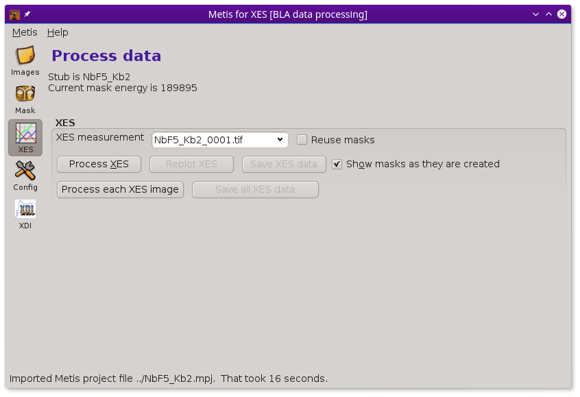
Once you have established a recipe for mask creation, you are ready to begin processing your resonant or non-resonant XES images. Clicking on the Data icon in the tool bar shows this page.

METIS's data processing tool.

Note that the Data icon has the same label as the mode in which METIS was invoked. In this case, it was involked in XES mode, so the label says XES.

In XES mode, the only set of controls shown are those related to computing and displaying XES spectra. See below for examples of METIS in HERFD or XES mode.

The drop down menu at the top of the XES box is filled with the contents of the Image files list from the Files page. Clicking the Process XES button processes the XES images one at a time using the mask recipe from the Mask page.

When clicked on, the Reuse masks button tells METIS to reuse the set of masks calculated at each elastic energy when processing the current image file. It takes a few 10s of seconds to work through the entire list of elastic energies. However, reapplying a set of calculated masks to a new image takes only a fraction of a second. Clicking this button off will force a recalculation of the entire set of masks.

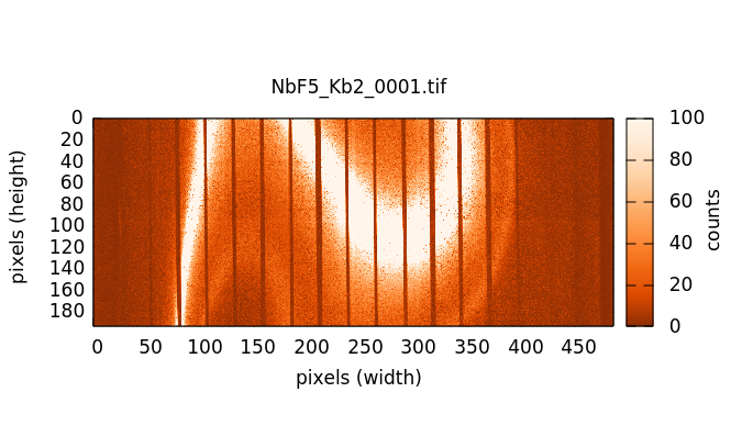
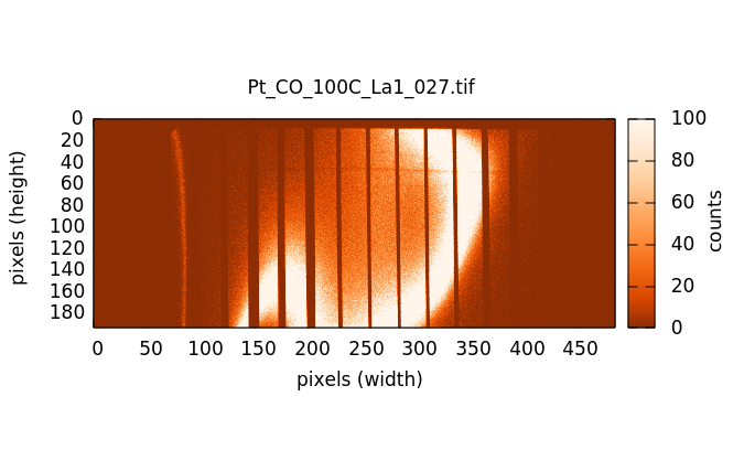
The XES image measure on NbF₅. The Kβ_1,3 is the bright stripe in the image. The distinct, but much dimmer stripe to the bottom and right of the image is the Kβ_2,5. The Kβ″ signal is in the broad, diffuse signal between the two peaks. The vertical stripes are from the Soller slits used to help suppress scattering from elsewhere in the beam path, thus reducing the background signal.

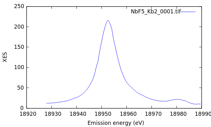
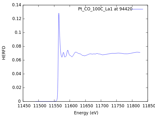
The XES spectrum computed for NbF₅. The Kβ_1,3 is the large peak at 18952 eV, the The Kβ_2,5 is the smaller peak at 18980 eV. The Kβ″ is the sort-of-shoulder above 18960 eV.

The Replot XES button will replot the current image file, reapplying the masks if required. The Save XES data button will prompt for a file name, then write the XES data from the current image as an XDI file. The columns of that file are energy, computed XES, number of illuminated pixels in each mask, and the unscaled signal at each energy.

The Process each XES image button will calculate the set of masks then apply them to each of the measured images. It will also compute the average of the XES spectra then plot each measurement along with the average. The Save all XES data button will write out the entire set of XES data to an XDI file. The columns are energy, average XES, number of illuminated pixels in each mask, followed by one column for each individual XES measurement.

Scaling the XES measurement

The reported XES spectrum is scaled by the number of illuminated pixels in the mask. The mask is multiplied by the XES image and this product is summed. That yields the photon count in those pixels falling under the mask at each energy. However, there is a significant discrepancy in the number of pixels actually illuminated at each energy. This has to do with the details of the geometry of the spectrometer and how each energy interacts with the analyzer crystal.

To approximate this geometry effect, each raw photon count is scaled by the number of pixels involved in the measurement. The elastic mask with the largest number of illuminate pixels has a scaling factor of 1. All other masks are scaled by N_pixels / N_largest. Elastic energies with relatively small illuminated pixel counts are scaled up to approximately remove the effect of geometry.

HERFD measurements

When starting METIS in HERFD mode, the Data tool displays several more controls.

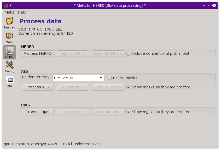
METIS's data processing tool in HERFD mode.

A HERFD data set includes elastic images measured over a range of energies surrounding a Kα, Kβ, Lα, or Lβ peak, including the top of the measured emission line.

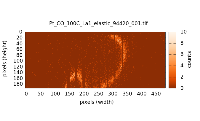
The image for 9442 eV, the top of the Pt Lα₁ line in a HERFD measurement on a Pt nanoparticle.

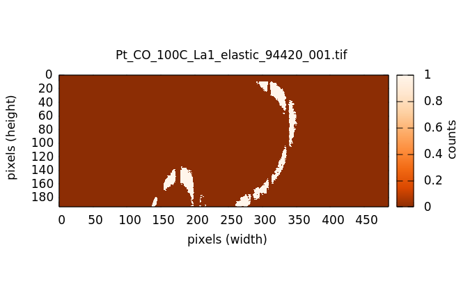
The mask for the 9442 eV image, processed with a bad/weak step with parameters 400/1 and a Gaussian blur with a threshold of 1.4.

The actual HERFD measurement involves measuring XES images at a range of energies corresponding to a conventional XANES scan. Below the edge (left image below) there is very little fluorescence in the image. As the scan goes through the edge and into the EXAFS, the fluorescence signal in the images grows, becoming quite bright with the brightness oscillating through the EXAFS wiggles.

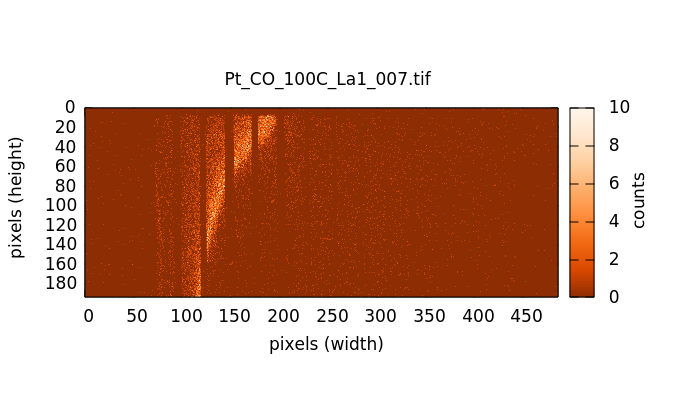
The Pt XES image at an energy in the XANES pre-edge.

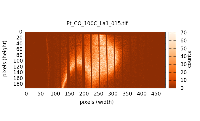
The Pt XES image at an energy somewhere in the middle of the XANES edge.

The Pt XES image at an energy above the Pt L₃ edge.

When the Process HERFD button is pressed, the mask is applied to each of the XES images over the XANES range. The signal under the mask is the HERFD signal at each energy.

The Pt HERFD computed from the sequence of XES images using the 9442 eV mask.

If the scan file contains an obvious column for a conventionally measured spectrum (either transmission or fluorescence with, say, a silicon drift detector), the conventional spectrum will be overplotted if the Include conventional mu(E) in plot button is checked.

The HERFD data can be replotted by clicking on the Replot HERFD button. Clicking on the Save HERFD button will prompt for a file name, then save the HERFD data as an XDI file.

The XES controls work much the same as when METIS is in XES mode. However, the XES spectra are unlikely to be all that interesting. For one thing, a typical HERFD measurement uses a rather sparse grid through the emission line. In the case of the Lα₁ line shown here, the emission line is so far below the Fermi energy, that the XES is unlikely to show anything of chemical interest. In the case of HERFD from a valence band or a Kβ_1,3 line, examining the XES at one or more energies might be a lot more interesting.

The RIXS controls work differently in HERFD mode than in RXES mode. In the case of HERFD, measuring the “RIXS” means to compute the HERFD spectrum at each measured elastic energy. The Process RIXS button will compute the mask at each elastic energy and apply it to the sequence of XES images throughout the XANES energy range.

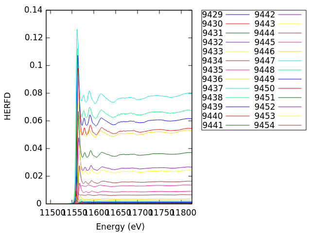
The Pt HERFD computed from the sequence of XES images using the each mask.

Here we see the dispersion of the edge of the HERFD spectrum as we scan through the Lα₁ line using the sequence of masks. The signal is largest at 9442, the top of the Lα₁ line, and is quite weak in the tails of the line.

The Replot RIXS button redisplays this image. The Save RIXS, saves this ensemble of spectra as an ATHENA project file.

Summing these HERFD spectra, weighted by the number of illuminate pixels in each mask, results in a spectrum that resembles a conventional XANES spectrum. In essence, making this sum introduces the core-hole broadening associated with the emission line. Try summing up the spectra from the project file in ATHENA and comparing with a conventional measurement. They won't be identical, but they will be close.

RXES measurements

When starting METIS in RXES mode, the Data tool displays controls for computing the RIXS plane.

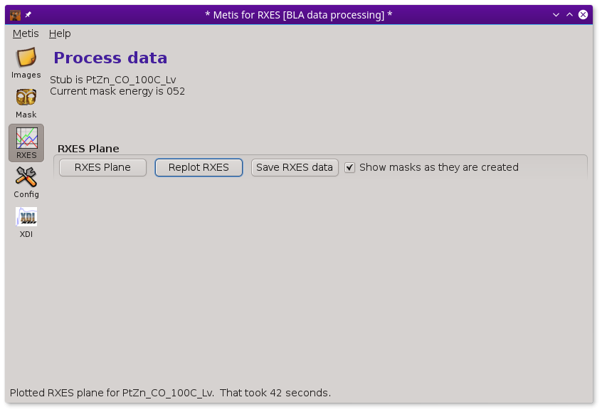
METIS's data processing tool in RXES mode.

This calculation is, in a certain sense, much like the RIXS calculation in HERFD mode, but the result is organized in a different way. In the HERFD-mode RIXS calculation, the intent is to examine the HERFD with the spectrometer set to different emission energies. In RXES-mode, the intent is to make a surface plot of the RIXS plane. Here is the result of the RXES-mode calculation.

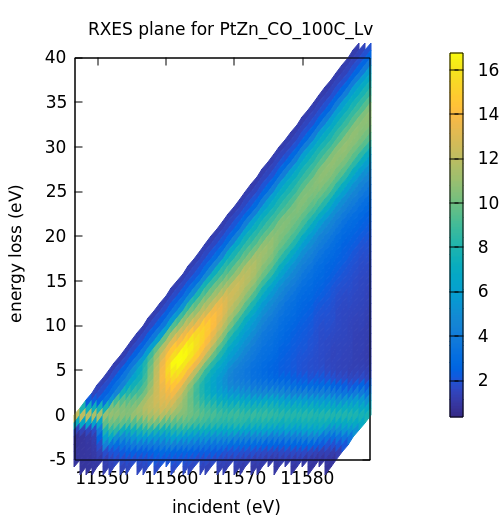
The result of the RXES calculation for the valence band emission near the Pt L₃ edge.

This is a visualization format that is common in the RIXS literature, plotting energy transfer as a function of incident energy. Energy transfer is E_incident - E_emission. The stripe at 0 on the y-axis, then, is the elastic signal. The RIXS signal is the diagonal stripe.

The Replot RXES button redisplays this surface plot. The Save RXES, saves the surface plot data as a Gnuplot block data file.

The color scheme is controlled by the ♦metis→splot_palette_name configuration parameter. There are about 80 options for this color palette. Many of them are perceptually improved colormaps, but some widely popular (but truly horrible) options exist – like the common Jet (aka rainbow) colormap. But honestly, just because “Jet” is a choice doesn't mean that you have to choose it....

See the chapter on data visualization for a complete listing of colormap options.

---

Xray::BLA and METIS are copyright © 2011-2014, 2016 Bruce Ravel and Jeremy Kropf – This document is copyright © 2016 Bruce Ravel

This document is licensed under The Creative Commons Attribution-ShareAlike License.

If this software and its documentation are useful to you, please consider supporting The Creative Commons.