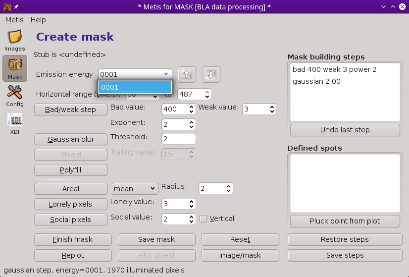
The Mask tool¶

At the top of the mask creation tool is a drop-down menu showing the entire list of measured elastic energies. In xes and rxes mode, the lowest elastic energy value is displayed initially. In herfd mode, the energy closest to the energy of the element and line displayed on the Files tool is initially selected.

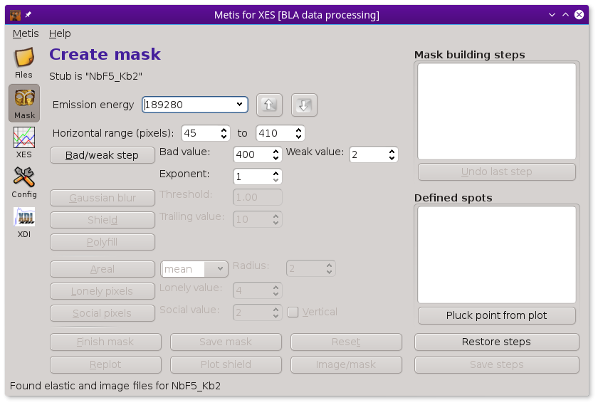
METIS's mask creation tool.

The purpose of this tool is define how the images measured at each elastic energy will be turned into a mask that can then be used to interpret the actual measurement.

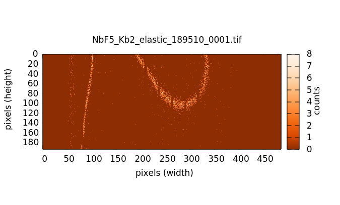
Here is an example of mask creation for the elastic measurement at 18951 eV on NbF₅:

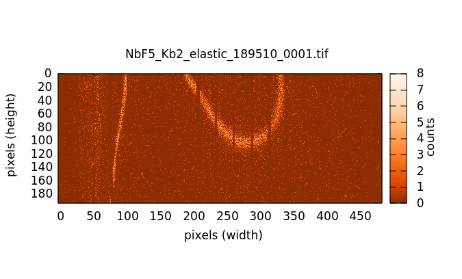
The measurement of the elastic scattering at 18951 eV on the NbF₅ sample.

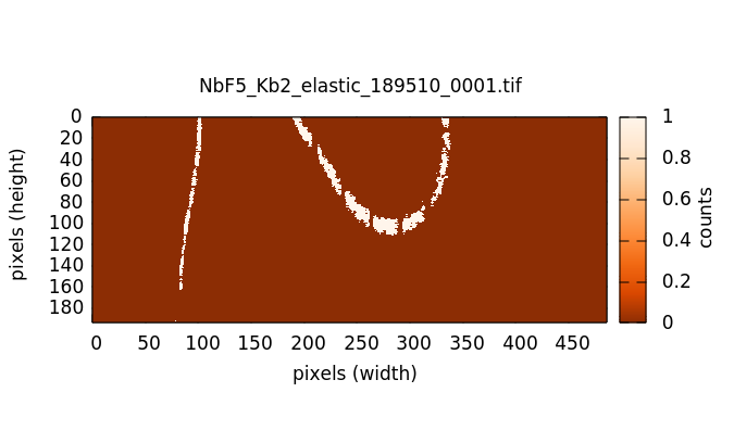
A plausible mask for the 18951 eV measurement on the NbF₅ sample. This was made using the bad/weak and Gaussian blur mask creation steps.

The end result of mask creation is a simple image wherein each pixel has either a 0 or 1 value. The 1-valued pixels represent the pixels illuminated by photons of a given energy, in this case 18951. When the Nb XES is measured either resonantly or non-resonantly, photons of energy 18951 will scatter through crystal in the spectrometer in the direction of one of those pixels on the detector.

The XES image will be multiplied pixel-by-pixel by the mask. The pixels outside the mask will be set to 0. The pixels within the mask are summed and will represent the Nb XES signal measured at that energy.

Here is how METIS's mask creation tool looks when the mask shown above is plotted:

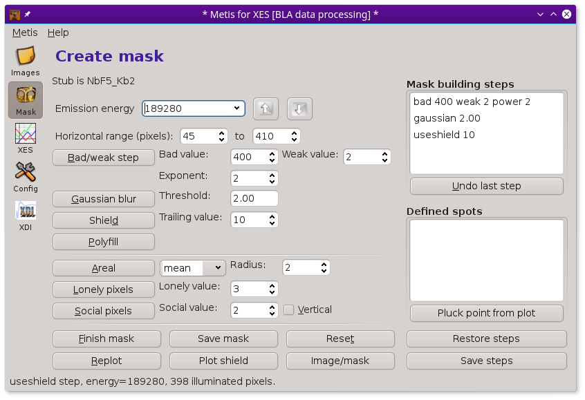
METIS's mask creation tool with the steps for the creating the mask shown above.

Each step of mask creation is taken by pressing the associated button. Many of the buttons have parameters which can be set by the user. In this example, the Bad/weak step and Gaussian blur buttons were clicked. Each step is written with is parameters in the Mask building steps list on the right side of the window. As each button is pressed, the plot of the elastic image is displayed with the result of the sequence of the mask creation steps.

The bad/weak step¶

The purpose of this mask creation step is to remove obviously spurious pixels. The Bad value indicates a pixel value which is anomalously high, either due to a dead pixel in the camera, a diffraction peak from the sample hitting the detector, or anything else that causes a very high valued pixel. All pixels above the bad value – in this example the bad value is 400 counts – will be set to 0 in the mask. In this way, bad pixels will not affect the resulting spectrum.

The weak value is an attempt to remove the low, fuzzy signal all around the periphery of the image. The assumption is that the pixels representing the elastic scatter will each contain several counts. Other pixels illuminated by stray photons are unlikely to have more than one or two counts.

Here is how the mask appears after applying the bad/weak step. It does a pretty good job, but leaves a lot of spurious pixels that obviously are not part of the mask.

The 18951 eV measurement after applying the bad/weak step.

The threshold value for bad and weak pixels are set using the controls to the right of the Bad/weak step button. The controls above for the Horizontal range are also used in the bad/weak step. By examining the elastic images from the lowest and highest energies, you can define region at the ends of the images which are never used in the measurement. In the bad/weak step, the pixels to left of the lower value of Horizontal range and to the right of the upper value will be set to zero, thus eliminating any spurious points from any mask that might make it through any of the mask creation steps.

Finally, the Exponent control is used to set the value for the exponent used to raise the elastic image to some power. This is done after the bad and weak pixels are removed. The point of this is to enhance the contrast in the case of weak elastic scattering. When you have a strong elastic signal, an exponent of 1 should suffice. Note that changing the changing the exponent value will have an effect on the appropriate value of the Gaussian threshold, described below.

The Gaussian blur step¶

This step performs a two-dimensional convolution with a pseudo-Gaussian kernel. The kernel can be of size 3 pixels by 3 pixels or 5 by 5. This is set by the ♦metis→gaussian_kernel configuration parameter. The 3x3 kernel is

1/16	2/16	1/16
2/16	4/16	2/16

1/16	2/16	1/16

The 5x5 kernel is

1/271	4/271	7/271	4/271	1/271
4/271	16/271	26/271	16/271	4/271
7/271	26/271	41/271	26/271	7/271
4/271	16/271	26/271	16/271	4/271
1/271	4/271	7/271	4/271	1/271

At each pixel, this kernel is multiplied by the surrounding pixels. The result is summed and the kernel is set to that summed value. This has the effect of suppressing pixels that do not have illuminated neighbors while preserving those that do.

The threshold value to the right of the Gaussian blur button is used as a cut-off. Pixels above that threshold are preserved in the mask and set to 1. Pixels below that threshold are rejected and set to 0.

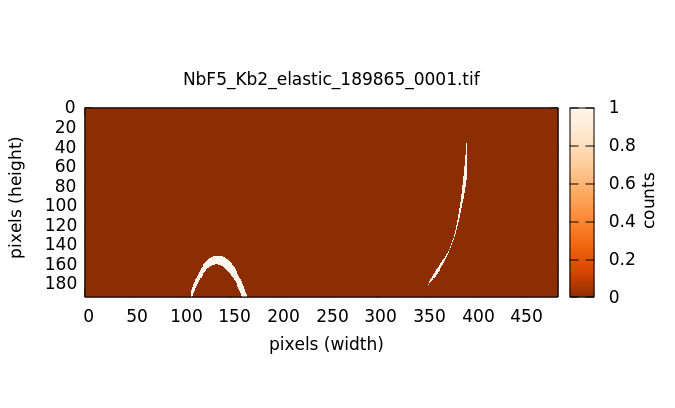
Here is the 18951 eV mask after a 5x5 Gaussian blur:

The 18951 eV measurement after applying the Gaussian blur step.

Shield step¶

The Kβ_2,4 emission lines being measured in this experiment is very close to the absorption edge. Towards the end of the sequence of elastic energies, the elastic signal is being measured very close to the absorption edge energy. Because Nb has a large core-hole broadening, a significant amount of fluorescence from the Kβ_2,4 lines themselves begins showing up in the elastic measurements. Here is an example at 18986.5 eV (as compared to the Nb⁰⁺ edge energy of 18986 – the edge for Nb⁵⁺ would be a few volts higher).

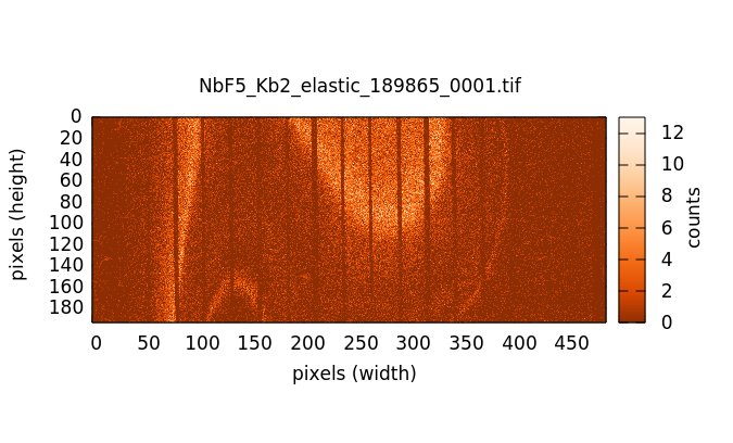
The 18986.5 eV measurement.

The elastic signal is the swoop towards the bottom and right of the image. The brighter signal near the top and left is the Kβ₂ signal beginning to appear due to the core-hole broadening.

The problem with the portion of the measurement coming from the Kβ₂ signal is that the Gaussian blur filter won't distinguish between it and the elastic signal. Indeed, the fluorescence part of the image is likely to be brighter than the elastic portion as we get close to the edge.

There is a simple heuristic for distinguishing the elastic from the fluorescence. Any pixels in the image that were part of earlier masks must not be part of the current mask. Using a succession of earlier masks, we can make a shield of pixels covered by earlier emission energies and use that shield to remove pixels from the current mask.

Because the energy resolution is typically larger than the step size, successive masks overlap somewhat. The parameter associated with this mask creation step defines how many energy steps prior to the current should be used to add to the shield. In this case the parameter is 10. Thus a shield is created by overlapping all the masks from the initial energy to 10 energy steps prior to the current energy. In this example, that results in a big blob covering the top and right portions of the image, as seen in the second image below.

The illuminated pixels in the shield are set to zero in the mask, resulting in the mask shown in the third image below.

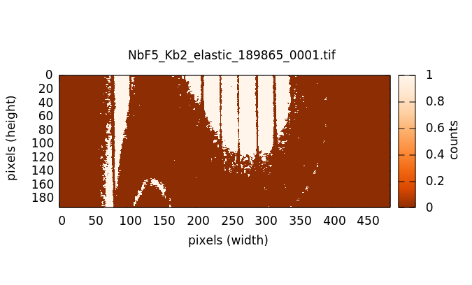
The mask 18986.5 after the bad/weak and Gaussian blur steps. The signal from the Kβ₂ remains in the mask as it easily passes the Gaussian blur threshold.

The shield created from all the masks 10 energy steps before the current energy and earlier.

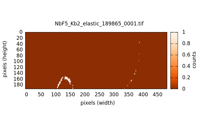
The mask after removing the pixels covered by the shield.

The use of the shield makes it possible to distinguish the elastic signal from the fluorescence. However, the elastic signal is pretty weak and relatively few pixels are left behind in this example.

The polyfill step¶

In an effort to improve upon images which are sparse after the mask creation steps already described, like the one shown above at 18986.5 eV, METIS offers a filling algorithm. In each column of the image, the top-most and bottom-most pixels remaining after the earlier steps are identified. A polynomial is fitted to the set of top-most points and another polynomial is fitted to the set of bottom-most points. These two polynomials are extrapolated over the range which includes the left- and right-most points used in the polynomial fits. All pixels between the two extrapolated polynomials (in the vertical direction) are illuminated.

The default is to use a polynomial of order 6. The ♦metis→polyfill_order parameter controls the order used. In the example below, polynomials of order 8 were used.

The mask after removing the pixels covered by the shield.

The mask after fitting polynomials or order 8 and illuminating the pixels between the polynomials.

This mask building step is helpful in situations where the mask is sparse. It will add many more pixels to the evaluation of the emission image. However, the curvature of the polynomial is might add additional pixels to the mask. Also any spurious points remaining in the mask will severely impact the quality of the fitted polynomials.

The polyfill algorithm presumes that the polynomials will be analytic functions. If the elastic signal “loops” on itself such that for a given column in the image, there are two distinct, vertically displaced regions of the mask, then the polyfill will fail rather dramatically.

When using the polyfill step, it is prudent to examine each mask individually and use the step removal algorithm described below wherever necessary.

Other mask creation steps¶

There are three more mask creation steps that can be added to the mask creation recipe. Each of them is similar to the Gaussian blur, but with certain differences.

The areal mean step takes a “radius” parameter. It uses an n-by-n (where n is twice the parameter value +1, thus radius 2 is a 5x5 kernel) uniform kernel to make a convolution of the image.
The lonely pixel step removes any pixels from the mask that do not have enough illuminated neighbors.
The social pixel step includes any pixels into the mask that are not illuminated, but which have a sufficient number of illuminate neighbors. This step is useful for filling in gaps in a mask, but has the negative side effect of making the mask wider, thus decreasing energy resolution.

If the vertical button is pressed, then the social check is only made in the vertical direction. In that case, the socail value should be 1 or 2 or the step will have no effect.

The mask building steps list¶

In the upper right corner of the Mask tool is a list box containing the mask building recipe. As you click buttons for the various mask building steps, the steps and any associated parameter values are written to the list.

Step buttons can be clicked in any order, thus adding steps to the recipe in any order. When the XES data is processed, the mask recipe will be applied as listed to each emission energy image in sequence.

You can move backwards through the recipe by clicking the Undo last step button. This removes the last step from the list, then reprocesses the image with the remaining recipe steps. In this way, it is easy to test different parameter values against your actual elastic images.

Defining spots in images¶

In the measurement at 18960 eV, there are a couple of bright spots in the fuzzy bit on the left due to the early appearance of the fluorescence signal. These two spots are at (60,12) and (60,158).

Processing to the point of the Gaussian blur filter leaves spots in the image that are obviously removed from the elastic signal.

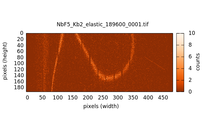
The measured elastic image at 18960 eV.

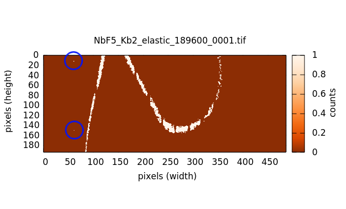
The mask after application of the bad/weak and Gaussian blur steps. The two spurious points are indicated by the blue circles.

There are two problems with these spurious spots. First, they will add signal to the measured XES at 19860 that should not be there. Also these spots will have a profound impact on the polyfill step. Here is what the polyfill step looks like on these data:

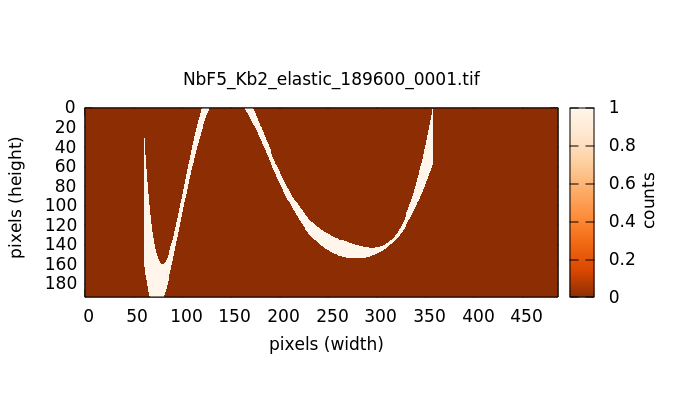
The effect of outlier points on the polyfill mask creation step.

This is obviously wrong.

There are several ways of dealing with spurious spots like this.

In this case, since the spots arise from fluorescence, the shield step will be effective at removing them. However, spots are often due to diffraction from the sample, in which case the shield is not guaranteed to be effective.
Raising the Gaussian blur threshold also might work. Indeed, in this case, raising the threshold to 1.2 is sufficient for removing those two spots. Again, diffraction peaks are not amenable to removal by the Gaussian blur filter as they are often quite strong compared to the level of the elastic signal.
Also the lonely pixels step with a value of 2 is sufficient to remove these spots.

With those spots removed, the polyfill step works as expected.

If you have tried all those tricks and you are unable to remove the spots while retaining significant area in the mask, it is time for a more hands-on approach. For situations where other mask creation steps don't work well, METIS allows you to select a specific point in a specific elastic image and remove it from the mask.

When you click on the Pluck point from plot button, you are prompted to double click on a spot in the image. When you do so, the point plucking dialog is posted.

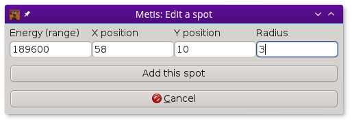
The point plucking dialog.

In this example, the point (58,10) is selected for energy 18960.0 eV. Because it can be hard to hit the exact right point and because these spots might be much larger than a single pixel, you are prompted for a radius. 3 is the default and is often is quite big enough to fully cover a spot. In the example below, a radius of 10 was used along with a weak pixel value of only 1 so that the effect of defining a point is clearly demonstrated.

The elastic image at 18960 eV with a large spot centered at (58,10) plucked out.

When the bad/weak step is processed along with the horizontal range, the list of spots is examined and any spots defined for the current elastic energy are also set to zero in the image, as seen above in the upper right part of the plot.

While this method of removing spurious spots can be quite tedious, it gives very fine-grained control over spot removal in an ensemble of data. For a situation where the elastic signal is not much bigger than the background, manual spot removal might be your only choice.

Right clicking on the defined spots list posts a context menu which can be used to edit or remove individual points from the list or to clear the list entirely.

All the rest of the buttons¶

Finish mask

Some mask creation steps may leave pixels with values other than 0 or 1. This step is a final pass to verify that any non-zero pixels are set to unity. This will be added automatically to the recipe in the steps list before data are processed in the Data tool.

Save mask

Save a mask as an image file.

Reset

Empty out the mask building steps list and restore parameters to their default values.

Replot

Replot the mask for the current energy.

Plot shield

Plot the shield for the current energy, if the shield step is being used.

Image/mask

This is a toggle button. When toggled on, it shows the raw image for the current energy. When toggled off, it replots the mask according to the current recipe.

Restore steps

Restore steps and spots from a save file.

Save steps

Save the current recipe of steps and spots to a save file.

RXES measurements¶

The RXES measurement uses a single set of images both for making masks and as the measured data. The trick is to distinguish the elastic portion of the image from the fluorescence portion.

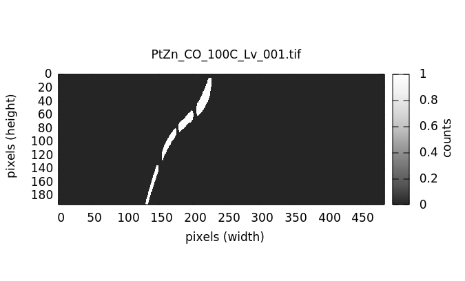
The shield step in the mask creation process is key to this. Here are the masks generated from the example images shown in the explanation of the Files tool.

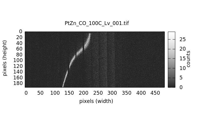
A Pt RXES image at a low energy.

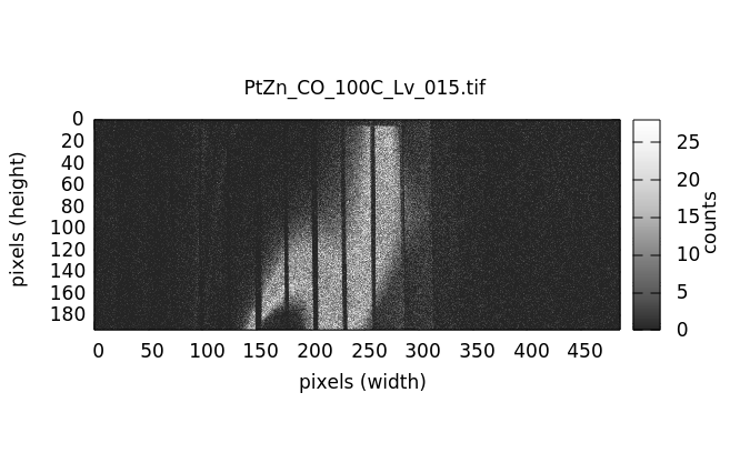
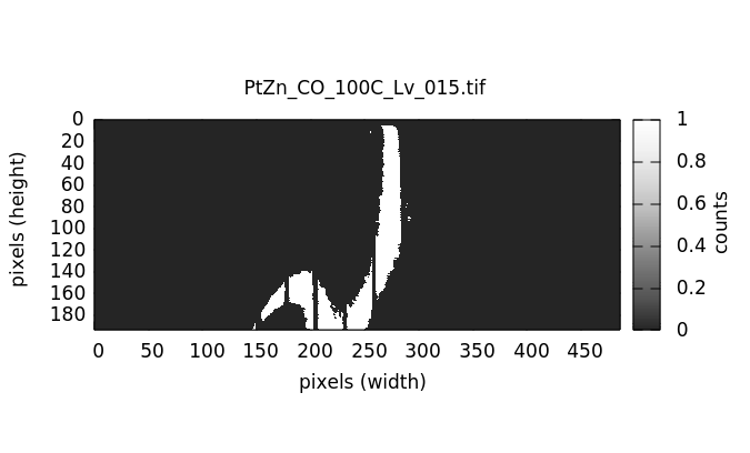
A Pt RXES image in the middle of the image sequence.

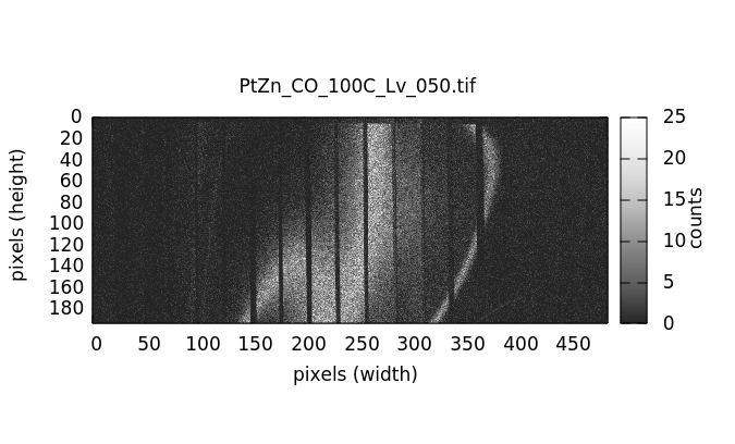
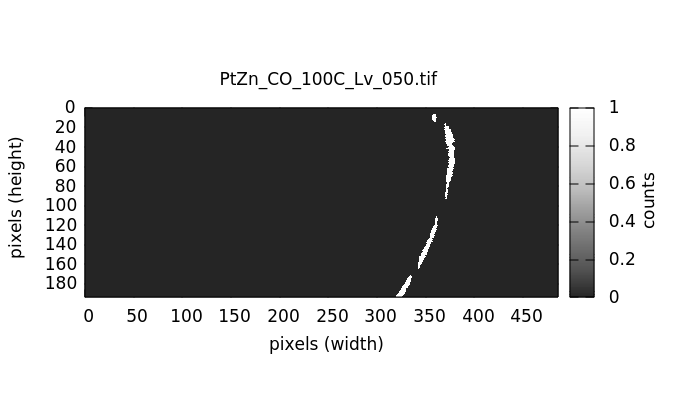
A Pt RXES image at the end of the image sequence.

The corresponding mask for the Pt RXES image at a low energy.

The corresponding mask for the Pt RXES image in the middle of the image sequence.

The corresponding mask for the Pt RXES image at the end of the image sequence.

The recipe for these masks is bad/weak with parameters 400/1/1, a Gaussian blur filter with a threshold of 6.0, and a shield step with a parameter of 5. That is, the masks from 5 steps back and prior are used to construct the shield which removes the fluorescence signal from the mask. The part that remains is a reasonable extraction of the elastic signal. The reason the shield step with a parameter of 5 can be trusted is that the mask from the end of the image sequence is a fair representation of the stripe that corresponds to the elastic signal.

This sequence of masks will then be applied to the same sequence of images to extract the resonant XES signal at each energy.

Examining a single file¶

When started in mask mode, the Mask tool is mostly the same as in other modes.

METIS's mask creation tool in mask mode.

The Emission energy list has only a single entry and the shield step is disabled. Otherwise, everything works the same. The big difference is that the Data tool is not shown in mask mode. The purpose of mask mode is to play around with the mask creation algorithm using an individual file.

This document is licensed under The Creative Commons Attribution-ShareAlike License.

If this software and its documentation are useful to you, please consider supporting The Creative Commons.