Setting math expressions

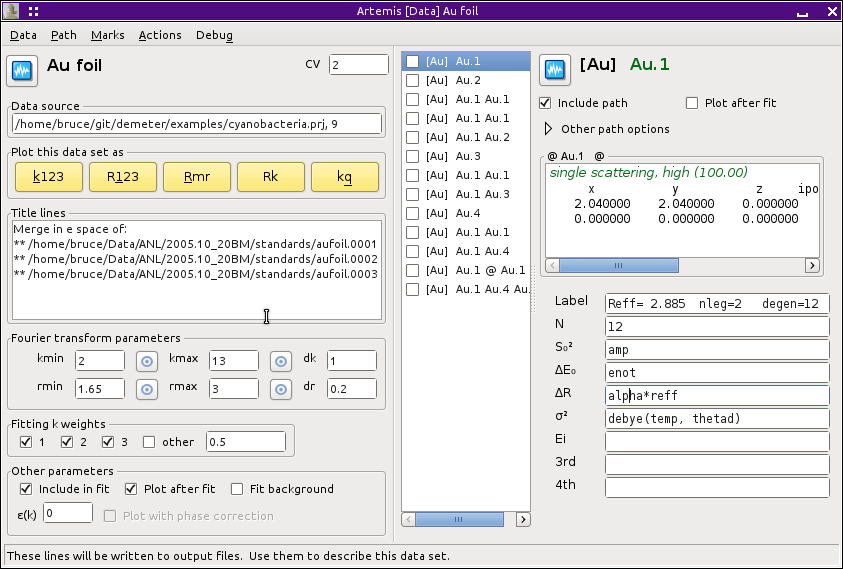
Once some paths have been dragged from the FEFF window onto the Data window containing the gold foil data, it is time to begin defining math expressions for the path parameters. In the following figure, the path corresponding to the first coordination shell has been selected from the path list. A path is selected by left clicking on its label in the path list. Doing so, displays that path on the right side of the Data window.

At the top of the Path page are two checkboxes. One is used to include and exclude a path from the fitting model. In this way, you can control which paths are used in a fit without having to remove them from the path list. The other check box is used to indicate if the current path should be transfered to the plotting list in the Plot window at the end of a fit.

Implement and explain the two items in the “other path options” pane.

The text box contains a brief description of the geometry of the scattering path. For a path with degeneracy greater than 1, the scattering geometry of one of the degenerate paths is shown. The simple explanation of the shape of the path and its heuristic importance are also given in the text box.

Implement a way to display a text box which shows all the paths contributing to the degeneracy + report on fuzziness of the degeneracy.

Beneath the scattering geometry is a table of path parameters labels and text boxes. Math expressions are entered into these text boxes.

In the preceding image, a simple fitting model appropriate for a cubic, monoatomic material like our gold foil has been entered for the first shell path. This includes simple expressions for S²₀ and E₀ consisting of variables that will be floated in the fit. A model of isotropic expansion is provided for ΔR. The σ² path parameter is expressed using the correlated Debye model. The other path parameter text boxes have been left blank and will not be modified in the fit.

This, of course, establishes the parameterization only for the first path. The same editing of path parameter math expressions must happen for all the other paths used in the fit.

The most straightforward way to do this editing chore is to click on each successive path in the path list, then click into each text box, then type in the math expressions. That, however, is both tedious and error-prone.

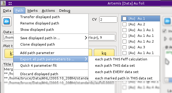
For math expressions that are the same for every path – E₀ is a common example – ARTEMIS provides some automation tools. Each of the path parameter labels on the Path page is sensitive to either left or right click. Either kind of click posts a menu like the one of the right. The top option is used to erase the contents of the associated text both, but only on this path.

The next four options are used to push the math expression for the associated path parameter onto other paths. These four options allow some control over the paths that are targeted to receive the pushed path parameter values.

The last two options are used to grab the math expression from one of the surrounding paths.

The menu that pops up for the σ² parameter has two additional options. One inserts a math expression for using the correlated Debye function for σ², the other inserts the math expression for an Einstein model. Both the Debye and Einstein functions depend on the measurement temeprature and a characteristic temperature. Typically, the measurement temperature is a set variable and the characteristic temperature is a guess. When either function is inserted into the text box, parameters are automatically created on the GDS page.

The Path menu on the Data page offers a way of pushing all the path parameters from the displayed path to other paths. The same options for targeting other paths are presented.