Marking and Plotting

The check buttons next to each path in the path list are central to many features in ARTEMIS related to plotting and other tasks. Along with all of the tools in the Mark menu, you can mark a group of paths by clicking elsewhere on the path list while holding down the shift key. Doing so marks all paths between the selected one and the one shift-clicked upon.

Control-clicking on the path list is also a special function used for two purposes. Doing a control-click starts a drag-and-drop with the path you click on. Dropping the path on another data window, copies If you drop the path on the same path list, that path to that Data set. Dropping the path on the same path list is equivalent to cloning the dragged path, with the clone being appended to the end of the path list.

Mistakenly control-clicking rather than shift-clicking will likely result in a path being cloned. This can be surprising and confusing, so take care!

Write a page about tools for building MDS fits

---

 

Moving paths to the Plotting list

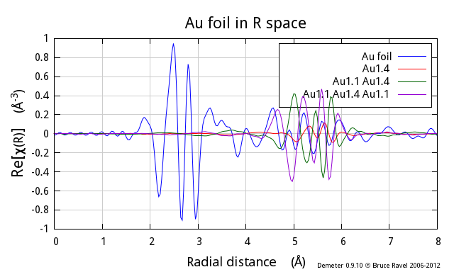
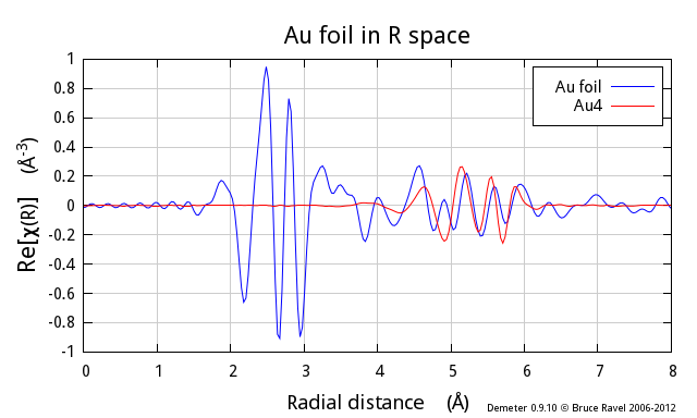
ARTEMIS has no special plot types involving individual paths like those for the data sets. Any plots with paths are constructed using the Plotting list on the Plot window. There are three ways of moving individual paths to the Plotting list.

1. The blue button with the squiggly line in the upper left corner of the Path page transfers that path to the Plotting list.

2. A path will be transferred automatically after a fit if its “Plot after fit” button is checked.

3. The set of marked groups will be transferred when “Transfer marked” is selected from the Actions menu. This is probably the most common way of constructing plots involving paths.

Another new feature in this version of ARTEMIS related to plotting is called a “virtual path”, or a “VPath”. A VPath is an ensemble of normal paths which are summed. The sum is then plotted in k-, R-, or q-space. A VPath is made by marking a set of paths then selecting “Make VPath from marked” from the Actions menu. VPaths are discussed in more detail the chapter on the Plot window.

When the VPath is created, it is placed in the VPath tab in the Plot window and in the Plotting list. The VPath list contains tools for renaming and discarding VPaths, displaying its constituants in the Main window status bar, and a VPath onto the Plotting list. (Remember that, unless the “Freeze” button is clicked, the Plotting list is cleared and repopulated after each fit.)

---

 

Phase corrected plots

When the Data page button labeled “Plot with phase correction”, plots using that data set and/or any of its paths will be plotted with phase correction. This means that the contributions of the central and scattering atom phase shifts will be removed before the Fourier transform. This has the effect of shifting the peaks in χ(R) by about +0.5Å, such that the first shell peaks at an R value close to the physical interatomic distance between the absorber and first shell scatterer.

The phase information is taken from one of the paths. Each path has a button labeled “Use this path for phase corrected plotting”. These buttons are exclusive – only one path per data set can have its button ticked on. The phase information from that path is used for the phase corrected plots.

If you turn on phase corrected plotting without having selected a path to use, ARTEMIS will issue a warning in te status bar and turn phase corrected plotting back off. You must select a path to use as the source of the phase information.

Note that, when making a phase corrected plot, the window function in R is not corrected in any way.

Also note that the phase correction propagates through to χ(q). While the window function will display sensibly with the central atom phase corrected χ(q), a “kq” plot will be somewhat less insightful because phase correction is not performed on the original χ(k) data.