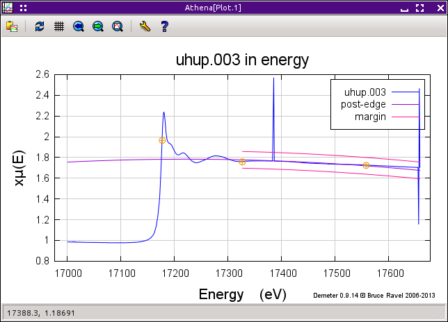
Deglitching and truncating data

Removing spurious points from your data

Deglitching

Occasionally your data has spurious points that are obviously different from the surrounding points. These so-called glitches can be caused by a variety of issues involving the monochromator, the electronics, or the sample itself. In principle, it should not be necessary to do anything at all about glitches. A feature in the data that is only one or two points wide necessarily contributes a high frequency signal to the data. Since the data are treated using Fourier techniques, these high frequency additions to the data should have scant impact on the data.

In practice, there are a variety of ways that glitches like those shown on the right in the figure below can impact the processing of the data. Certainly, large glitches are unsightly and have an aesthetic impact on the presentation of your data.

The process by which glitchy points are removed from the data is called deglitching. Yes, I also think that's a funny sounding word.

The deglitching tool.

ATHENA's approach to deglitching involves simply removing the points from the data. No effort is made to interpolate from the surrounding points in an effort to replace that point with a presumably more appropriate value. The reason that no interpolation is done is that EXAFS data are typically measured on a grid that is oversampled. When the data are converted from μ(E) to χ(k) as part of the background removal, the data are rebinned onto the standard k-grid. Since a rebinning is performed later in the data processing, there is no reason to interpolate at the time of deglitching.

Deglitching only removes points from the data in ATHENA's memory. The data on disk are never altered.

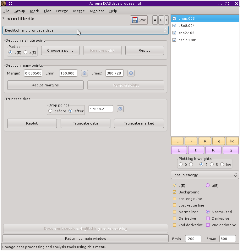
There are two methods of deglitching offered by ATHENA's deglitching tool, shown above. The first involves selecting and removing the glitches one by one. The points are selected by clicking the “Choose a point” button then clicking on the glitch in the plot. After clicking on the plot window, the selected point is indicated with an orange circle, as on the left of the next figure. Clicking the “Remove point” button removes that point from the data, shown in the bottom panel.

 
  
  

(Left) This is an example of data the needs deglitching. In this case, there was a problem with data channels not arriving at the measurement computer in the proper sequence. This timing problem resulted in occasionally spikes in the data. (Right) A point has been selected for removal. The point flagged for removal is indicated with a little orange circle. (Bottom) The selected point has been removed from the data. The deglitching margins are displayed along with the data.

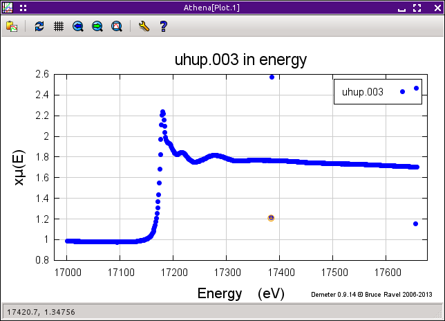
The second method for removing glitches is more automated. In the figure above, the deglitching margins are shown by the pink lines. Those margins are drawn between the specified minimum and maximum energy values. The lines are drawn a set amount above and below the post-edge line used to normalize the data. The separation between the post-edge line and the margins is given by the value in the tolerance box.

When you click the “Remove glitches” button, and points that within the energy range of the margins but which lie above the upper margin or below the lower margin are removed from the data. These margins can also be drawn in the pre-edge region using the pre-edge line. There is no way to use margins in an energy region that includes the edge.

This technique is handy in that it quickly removes many glitches in a situation like the one shown. It is very dangerous, however, if not used with care. If the margins extend into the white line region or are so tight around the post-edge line that the oscillatory structure crosses the margins, this technique will happily remove good points from the data. Set your margins well!

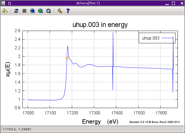
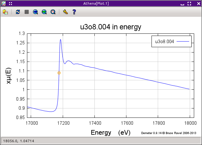
A useful variation of the point-by-point technique involves plotting the χ(E) data. This can only be done for glitches above the edge, but it can be a very useful technique for removing small glitches from the data. In this figure we see μ(E) data for U₃O₈ that appear fine.

 
  
  

(Left) μ(E) data for U₃O₈ that have a tiny glitch hidden in the high energy region. (Right) Plotted as χ(k), the glitch at about 12 Å⁻¹ in these χ(k) data is clearly seen. (Bottom) With potting as χ(E) selected. The spurious point at about 12 Å⁻¹ has been chosen.

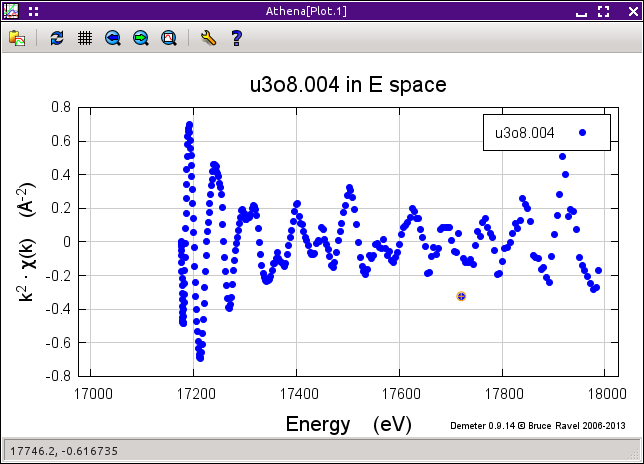
When the χ(E) is displayed, the k-weight value specified by the k-weight controls is used. From there, the point-by-point technique is identical to how it used with μ(E) data. The advantage is that small glitches might be easier to see and to pluck from the data when the data is plotted as χ(E). The point-by-point deglitching algorithm works on the χ(E) data in the same manner as for μ(E) data. Points are selected by clicking on the plot, then removed by clicking the “Remove point” button.

Truncation

If your data does something odd at one end of the scan, the easiest solution might be to simply trim it away. The truncation tool allows you to chop data before or after a selected value.

The radiobox is used to tell ATHENA whether points should be trimmed from before or after the selected point. The point can be chosen by typing in the box or by using the pluck button.

Tin oxide data with some spurious points near the end of the scan.

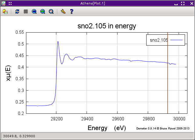
When you select a point, it is indicated with a vertical line, as shown in the plot above. To remove the data before or after that line, click the “Truncate data” button.

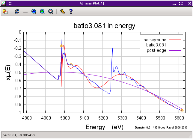
Sometimes the issue is not simply that the data are “icky” after a certain point. Sometimes your sample has elements with nearby edges, thus limiting the range over which you can actually measure the data. An example is shown in the next plot, the Ti K edge is at 4966 eV and the Ba L_III edge is at 5247 eV. A careless choice of spline and normalization range will lead to a data processing disaster.

The Ti K and Ba L_III edges of BaTiO₃.

Of course, truncation is not the only way of dealing with this issue. A careful choice of the spline, pre-edge, and normalization ranges is usually sufficient to treat any strange features at the beginning or end of the data set. So which is better? I think it's a matter of preference. As long as you understand what you are doing and process all your data in a consistent, defensible manner, you can use either approach.