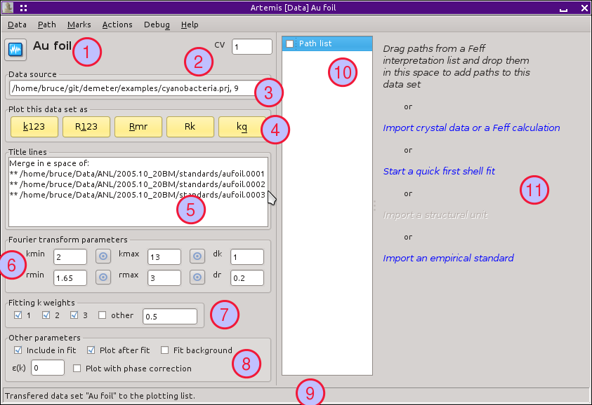
The Data window

After importing data from an ATHENA project file, several things happen:

1. A new Data window is created for interacting with that data set and the various controls are set to values taken from the ATHENA project file or from ARTEMIS' defaults.

2. A message is written to the status bar in the Main window.

3. The data are plotted in k-space.

4. The data are transferred to the plotting list in the Plot window.

5. An entry is placed in the Data list on the main window.

Here is the Plot window as it initially appears:

1. This button is used to transfer this data set into the plotting list in the Plot window.

2. This is the characteristic value of this data set. Typically, this is just incremented for each data set as it is imported. The CV can be used as a special parameter in math expressions.

3. This text box shows where this data set came from. Typically, this shows the fully resolved file name for an ATHENA project file, followed by the index of the data from that project file.

4. These five buttons generate special plots using this data set. Each of the special plots types is explained below. Like the Fit button from the main window, these buttons are recolored after a fit according to the value of the fit's happiness parameter.

5. This text box contains any title lines associated with the data.

6. These controls are used to set the functional form of the windows for forward and backward Fourier transforms. The R_min and R_max values are also used as the fitting range. The menus for selecting the windows functions are only displayed when the ♦Artemis → window_function is set to “user”.

7. These check buttons are used to set the k-weight values used to evaluate the fit. Note that these are check buttons and radio buttons not – more than one can be selected at a time. The default is that all of 1, 2, and 3 checked, resulting in a multiple k-weight fit. The default can be changed by editing the ♦Fit → k1, ♦Fit → k2, and ♦Fit → k3 parameters.

8. This area contains several other parameters related to this data set. When the first check button is checked, this data will be included in the fitting model. Unchecking it is a way of removing a data set from a multiple data set fit without actually disposing of the data. The second check button instructs ARTEMIS to automatically transfer this data set to the plotting list at the end of a fit. The third check button turns on background co-refinement. The ε text box allows you to specify a measurement error fit this data set. Finally, the last check button turns phase corrected plotting on and off. See the discussion of phase corrected plots.

9. This status bar is used to display messages specifically related to this data set. These messages are logged in the status buffer.

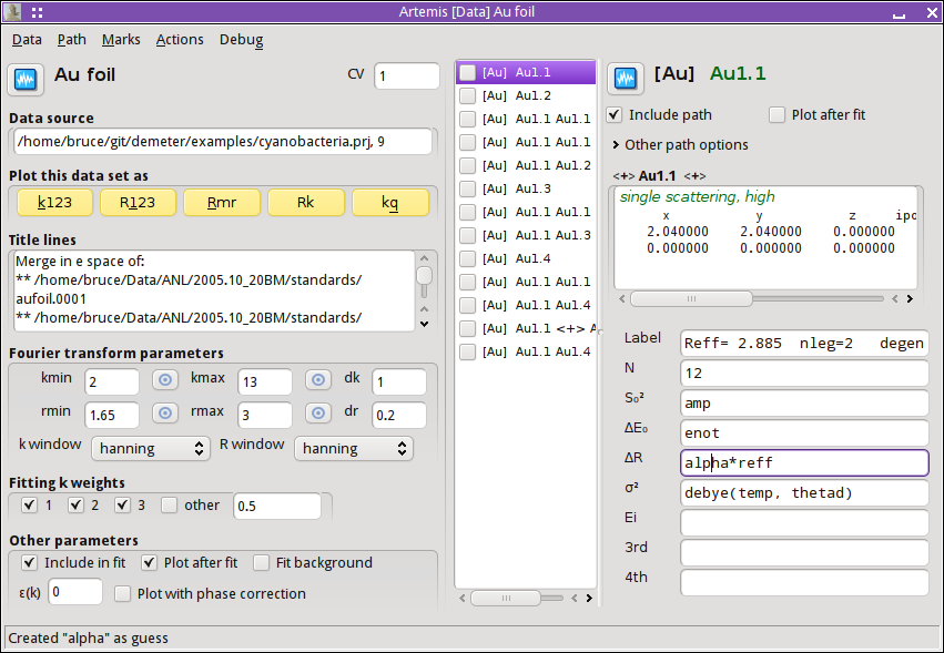
10. The paths list will become populated as paths are associated with this data set. How that works will be explained in the next chapter.

11. When no paths have yet been associated with a data set, this default page is displayed. The lines of blue text are sensitive to mouse clicks and initiate the import of certain kinds of data. All of those import options will be explained elsewhere in this document.

After one or more paths have been associated with this data set, the Data window looks something like this.

Note that the paths list is populated with the paths assigned to these data and that the right hand side of the Data window displays the details about a particular path. Clicking on an item in the paths list causes that path to be displayed on the right.

Note that each path in the path list has a check button associated with it. These check buttons are involved in much of the functionality described below.

Some vocabulary: The highlighted path is displayed on the right and is said to be selected. When a paths check button is checked, it is said to be marked. In this example, the first path is selected and no paths have yet been marked.

---

 

Special plots

The five plot buttons on the Data window make special plots of that data set along with its fit (if a fit has been run). Each of these is an elaborate, multi-component plot that cannot be made using the tools on the Plot window. The examples shown here are for a fit to gold metal out to the fourth coordination shell.

---

The k123 plot

This is the “k123” plot. It shows the data and fit as χ(k). Each k-weighting from 1 to 3 is shown. The data with k-weighting of 2 is plotted normally. The other two k-weightings are scaled by the appropriate number such that all three k-weighting appear to be about the same size in the plot. The Fourier transform window function is drawn over the k-weight of 1 spectrum.

---

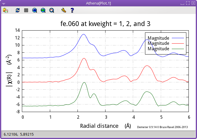
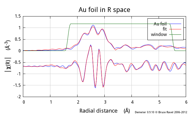
The R123 plot

This is the “R123” plot. It shows the data and fit as χ(R). The Fourier transform has been done with each k-weighting from 1 to 3. The data with k-weighting of 2 is plotted normally. The other two k-weightings are scaled by the appropriate number such that all three k-weighting appear to be about the same size in the plot. The back-Fourier transform window function is drawn over the k-weight of 1 spectrum to indicate the range over which the fit was evaluated (assuming the fit space is R, as is the default). The radio button in the Plot window for selecting the part of χ(R) is respected when this plot is made.

---

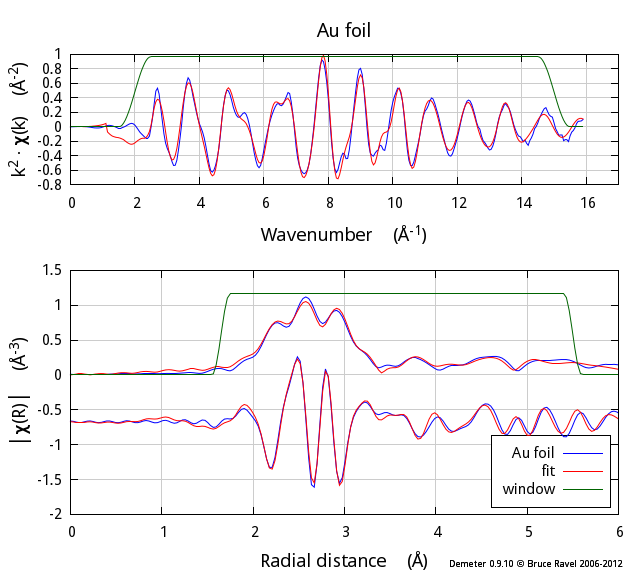
The Rmr plot

The “Rmr” plot is the plot displayed by default after a fit. It shows the magnitude and real part of χ(R) using the value of k-weighting selected in the Plot window. The back-Fourier transform window function is drawn over the magnitude spectrum to indicate the range over which the fit was evaluated (assuming the fit space is R, as is the default).

---

The Rk plot

The “Rk” plot is a stacked plot with the “Rmr” on the bottom and χ(k) on the top. The value of k-weighting selected in the Plot window is used. Fourier transform windows are drawn over the χ(k) and |χ(R)| spectra.

This is Bruce's favorite way of presenting data for publication. It is a compact representation of the data and the fit. All the interesting ways of visualizing the data and fit are presented on equal footing.

---

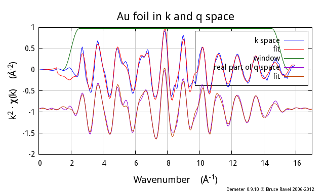
The kq plot

The “kq” plot shows the data and fit as χ(k) and χ(q). The value of k-weighting selected in the Plot window is used. The Fourier transform windows are drawn over the χ(k) spectra.

---

 

Data menu bar

---

 

The Data menu

This menu displays functions that can act on the data set displayed in that window.

Rename

Change the name of this data set. This is the name displayed next to the transfer button, in the plotting list, in the log file, and in plot legends.

Replace

Change the χ(k) by importing new data from an ATHENA project file. This is used to apply the current fitting model to a new data set.

Discard

Throw away this data set and its window. Also remove this data set from the Data list in the Main window.

Save data

Write this data set to a column data file. The χ(k) output option will write a file with columns for k, χ(k), k⋅χ(k), k²⋅χ(k), k³⋅χ(k), and the window function. The χ(R) output option will write a file with columns for R, the real part, the imaginary part, the magnitude, the phase, and the window function. The χ(q) option is of the same form a the χ(R) option.

Save data and fit

Write the data, the fit, and several other arrays to a data file in one of various forms of k, R, or q. This will have columns for the abscissa, the selected form of the data, and the corresponding forms of the fit, the background (if co-refined), the residual, the running R-factor, and the window.

Save data and paths

This will save the data along with each marked path to a column data file. The columns will be the same as for the data+fit output.

Other fitting standards

This submenu allows you to import a variety of special path types, including quick first shell paths and empirical standards. (Structural units have not yet been implemented in Artemis.)

Balance interstitial energies

(This feature has not yet been implemented in Artemis.)

Set all degeneracies

These two options allow you to control the degeneracy values of all the paths in the fit. The choices are to set them all to 1 or to have them all use their degeneracies from their respective FEFF calculations.

Set window function

When the ♦Artemis → window_function parameter is not set to “user”, this submenu will be displayed. It allows the user to change the window function to be used for both forward and backward Fourier transforms. Note that setting the window function in this way uses the same functional form for transforms in both directions. If you want to control the two functions independently (for some inscrutable reason), you must set ♦Artemis → window_function to “user”.

Export parameters

In a multiple data set fit, this allows you to constrain the data sets to have the same choice of Fourier transform parameters. (This feature has not yet been implemented in Artemis.)

Set kmax to Ifeffit's suggestion

Use IFEFFIT's suggestion for an appropriate value of k_max.

Show epsilon

Show the value of ε computed from the noise in this data set. The value will be displayed in the Data window status bar.

Show Nidp

Show the number of independent points computed from the Fourier transform and fitting range. The will be displayed in the Data window status bar.

---

 

The Path menu

This menu displays various functions that can be appied to the paths associated with this data set.

Transfer

Transfer the displayed path to the plotting list in the Plot window.

Rename

Change the name of the displayed path. This is the name displayed next to the transfer button, in the plotting list, in the log file, and in plot legends.

Show

Post a dialog box with IFEFFIT's current evaluation of all path parameters for the displayed path.

Save path

Write the displayed path to a column data file. The χ(k) output option will write a file with columns for k, χ(k), k⋅χ(k), k²⋅χ(k), k³⋅χ(k), and the window function. The χ(R) output option will write a file with columns for R, the real part, the imaginary part, the magnitude, the phase, and the window function. The χ(q) option is of the same form as the χ(R) option.

Clone

Make a copy of the displayed path and insert it into the path list. The degeneracies of the original and cloned path will be half the original degeneracy.

Add path parameter

Post the dialog on the right, which is used to add a path parameter math expression to multiple paths associated with this or other data sets. This is a convenience allowing you to edit the path parameters for many paths at the same time.

Export path parameters

Push the math expressions of each path parameter from the displayed path to other paths. This submenu has options for pushing these values to the other paths from the same FEFF calculation, to the marked paths, to all paths in this data set, or to all paths in all data sets.

Quick 4 parameter fit

This is a convenience function for setting up a simple, one-shell fit. Selecting this menu item will create 4 parameters in the GDS window and use those four parameters as the math expressions for S²₀, E₀, ΔR, and σ² for each path assigned to this data set. This is intended only for a one-path, one-shell fit. While it may be tempting to expect broader utility out of this function – don't. It really only serves this narrow purpose.

Discard

Discard the displayed path, removing its window, and removing it from the path list.

---

 

The Marks menu

Much of ARTEMIS' functionality revolves around groups of marked paths. This menu contains a number of shortcuts for marking paths. Note that each of these has a keyboard shortcut given on the right side of the menu. Learning the shortcuts for marking functions that you use frequently is key to the effective use of ARTEMIS.

Marking via these functions is cumulative. That is, most of them only add to the set of marked paths. Choosing to mark, say, all single scattering paths will not unmark any marked multiple scattering paths.

Several of these functions will post a dialog for receiving input. Marking by regular expression (regex) will prompt for a perl-style regular expression to match against the labels in the path list. The pattern you provide will be used only if it can be successfully parsed as a valid perl regular expression.

Marking either greater than or less than an A value will prompt for a cutoff in path ranking.

Marking either greater than or less than an R value will prompt for that R value.

Marking before or after the current path will mark those above or below the displayed path in the path list. Included and excluded refers to whether a path is selected as being included in a fit.

---

When using regular expression marking, you have access to perl's entire regular expression functionality. If you know what a “(?{ code })” extended expression is and you use it foolishly, you only have yourself to blame.

---

 

The Actions menu

Every item in this menu operates either on the set of included paths or the set of marked paths. Again, keyboard shortcuts are given in the menu.

The first two options will make a VPath out of either all the paths for this data set or the marked paths. The VPath will be placed in the plotting list in the Plot window and a plot will be made in R. The option to make the sum of all paths is particularly useful for comparing the fittingmodel to the data without actually running the fit.

The next two options will transfer paths to the plotting list, then make a plot in R.

The next two options will cause the set of marked paths to be included in or excluded from the fit. The next item computes the value of a bond valence sum using the set of marked paths. You will be prompted for some information about the absorber and scatterer.

The next item causes all marked paths to be discarded from your fitting project and removed from the path list.

The final two items are about controlling what gets transferred into the plotting list after a fit. The next to last item causes all marked paths to be transferred. The last item removes all paths from the list of things transferred

---

 

The Debug menu

This menu displays various dialog boxes showing aspects of the current state if IFEFFIT or ARTEMIS. These are mostly used for debugging purposes. This menu is only displayed if the ♦Artemis → debug_menus configuration parameter is set to a true value.

---

 

The Data help menu

This menu is used to display the sections on the Data window or the Path page from the document.