Understanding the quick first shell tool in Artemis

ARTEMIS offers several ways to get information from FEFF into a fitting model. One of these is called a quick first shell path. It's purpose is to provide a model-free way of computing the scattering amplitude and phase shift well enough to be used for a quick analysis of the first coordination shell.

The way it works is quite simple. Given the species of the absorber and the scatterer, the absorption edge (usually K or L_III), and a nominal distance between the absorber and the scatterer, ARTEMIS constructs input for FEFF. This input data assumes that the absorber and scatterer are present in a rock salt structured crystal. The lattice constant of this notional cubic crystal is such that the nearest neighbor distance is the nominal distance supplied by the user. FEFF is run and the scattering path for the nearest neighbor is retained. The rest of the FEFF calculation is discarded. The nearest neighbor path is imported into ARTEMIS with the degeneracy set to 1.

The assumption here is that the notional crystal will produce a scattering amplitude and phase shift for the nearest neighbor path that is close enough to what would be calculated by FEFF were the local structure actually known. Does this really work?

---

 

Using the quick first shell tool to model first shell data

To demonstrate what QFS does and to explain the constraints on the situations in which it can be expected to work, let's take a look at my favorite teaching example, FeS₂. Anyone who has attended one of my XAS training courses has seen this example.

These three figures show the S atom in the 1st coordination shell computed using the known crystal structure for FeS₂. This calculation is the blue trace. The red trace is the contribution from a S atom at the same distance as computed using the quick first shell tool. These calculations are plotted as χ(k), |χ(R)|, and Re[χ(R)].

 

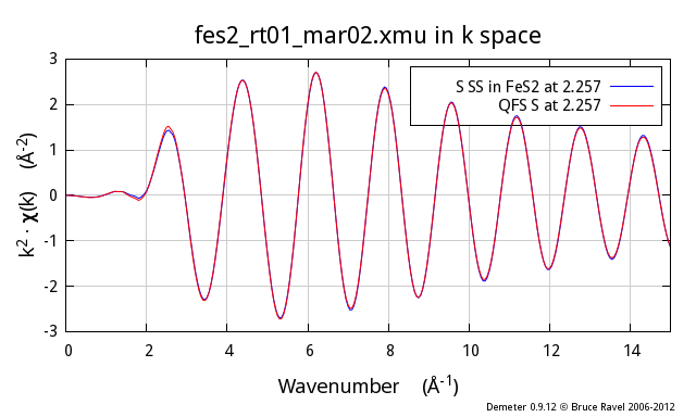
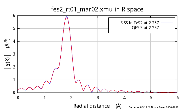
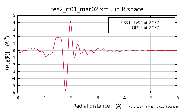
As you can see, these two calculations are identical. You cannot even see the blue trace underneath the red trace. It is clear that the QFS calculation can be substituted for the more proper FEFF calculation of the contribution from the nearest neighbor.

Why does this work?

FEFF starts by calculating neutral atoms then placing these neutral atoms at the positions indicated by FEFF's input data. Each neutral atom has an associated radius – the radius within which the “cloud” of electrons has the same charge as the nucleus of the atom. The neutral-atom radii are fairly large. When placed at the positions in the FEFF input data, these neutral-atom radii overlap significantly. This is a problem for FEFF's calculation of the atomic potentials in the material because it means that electrons in the overlapping regions cannot be positively identified as belonging to a particular atom.

To address this situation, FEFF uses an algorithm called the Mattheis prescription, which inscribes spheres in Wigner-Seitz cells, to reduce the radii of all atoms in the material together until the reduced radii are just touching and never overlapping. These smaller radii are called the muffin-tin radii. The electron density within one muffin-tin radius is associated with the atom at the center of that sphere. All of the electron density that falls outside of the muffin-tin spheres is volumetrically averaged and treated as interstitial electron density. All the details are explained in J.J. Rehr and R.A. Albers, Rev. Mod. Phys., 72, (2000) p. 621-654 (DOI: 10.1103/RevModPhys.72.621).

The scattering amplitude and phase shift is then computed from atoms that have a specific size – the size of the muffin-tin spheres – and with the electron density associated with those spheres.

The reason that the two calculations shown above are so similar is because the muffin-tin radii of the Fe and S atoms are almost identical. This should not be surprising. Either way of constructing the muffin tins – using the proper FeS₂ structure or using the rock-salt structure – start with Fe and S atoms separated by the same amount. The application of the algorithm for producing muffin-tin sizes ends up with nearly identical values. As a result the scattering amplitudes and phase shifts are nearly the same and the resulting χ(k) functions are nearly the same.

---

 

(Mis)Using the quick first shell tool beyond the first shell

This is awesome! It would seem that we have a model independent way to generate fitting standards for use in ARTEMIS. No more mucking around with Atoms, no more looking up metalloprotein structures. Just use QFS!

If you think that seems too good to be true – you get a gold star. It most certainly is.

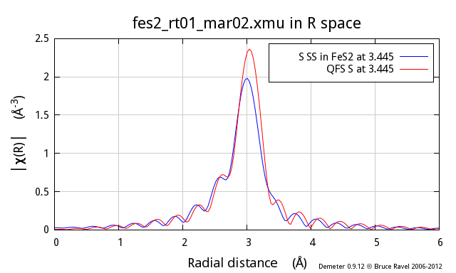
Following the example above, I now show the second neighbor from the proper FeS₂ calculation, which is also a S atom and which is at 3.445 Å. The red trace is a QFS path computed with a nominal distance of 3.445 Å. As you can see, there are substantial differences, particularly at low k, between the two.

 

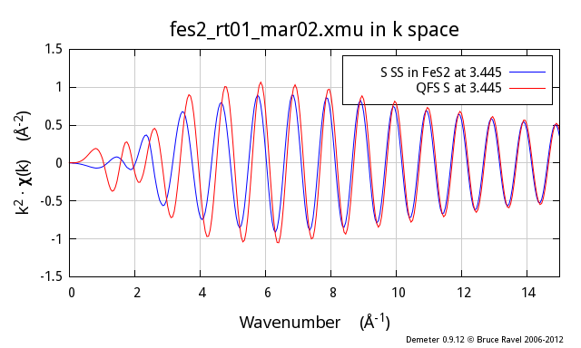
So, why does this not work so well? In the proper calculation, the size of the S muffin-tin has been determined in large part by the Fe-S nearest neighbor distance. This same muffin-tin radius is used for all the S atoms in the cluster. Thus, in the real calculation, the contribution from the second neighbor S atom is determined using the same well-constrained S muffin-tin radius as in the 1st shell calculation.

In contrast, the QFS calculation has been made with an unphysically large Fe-S nearest neighbor distance. Remember, the QFS algorithm works by putting the absorber and scatterer in a rock-salt crystal with a lattice constant such that the nearest neighbor distance is equal to the distance supplied by the user. In this case, that nearest neighbor distance is 3.445 Å!

The algorithm for constructing the muffin tins requires that the muffin-tin spheres touch. Supplied with a distance of 3.445 Å, the muffin-tin radii are much too large, the electron density within the muffin tins is much too small, and the scattering amplitude and phase shift are calculated wrongly.

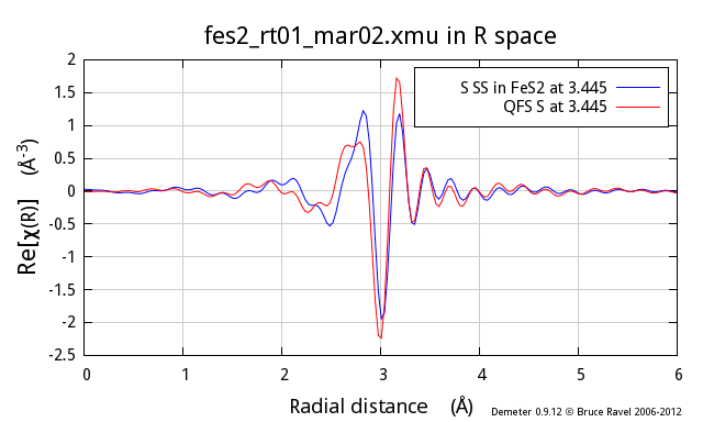
The central problem here is not that the red line is different from the blue line – although that is certainly the case and it is certainly a problem. The central problem is that, by misusing the QFS tool in this way, you introduce a large systematic error into your data analysis. This systematic error affects both amplitude and phase (as you can clearly see in the figures above). What's worse, you have no way of quantifying this systematic error. Your results for coordination number, ΔR, and σ² will be wrong. And you have no way of knowing by how much.

In short, if you misuse the QFS tool in this way, you cannot possibly report a defensible analysis of your data.

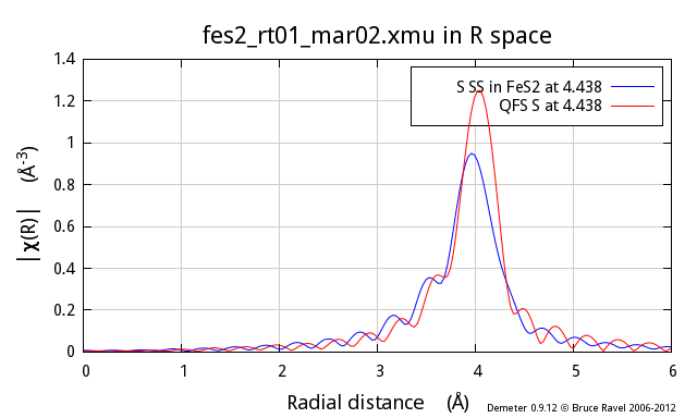
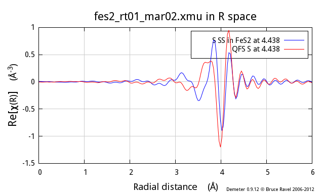
To add even more ill cheer to this discussion, the problem gets worse and worse as the nominal distance of the QFS calculation gets larger. Here I show the same comparison, this time for the fifth coordination shell in FeS₂, another S scatterer at 4.438 Å:

 

---

 

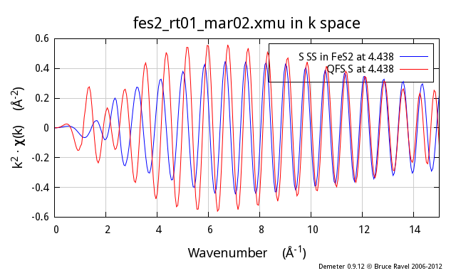
Executive summary

The quick first shell tool is given that name because it is only valid for first shell analysis.

If you attempt to use the QFS tool at larger distances, you introduce large systematic error into your data analysis. Don't do that!

---

 

So, what should you do?

Presumably, you have measured EXAFS on your sample because you because you do not know its structure. The point of the EXAFS analysis is to determine the structure. The upshot of this discussion would seem to be that you need to know the structure in order to measure the structure. That's a catch-22, right?

Not really. As I often say in my lectures during XAS training courses: you never know nothing. It is rare that you cannot make an educated guess about what your unknown material might resemble. With that guess, you can run FEFF, parameterize your fitting model, and determine the extent to which that guess is consistent with your data.

Crystalline analogs

In this paper, Shelly Kelly demonstrates how to use FEFF calculations on crystalline materials as the basis for interpreting the EXAFS of uranyl ions adsorbed onto biomass. In that paper, she shows the pH dependence of the fractionation of the uranyl ions among phosphoryl, carboxyl, and hydroxyl binding sites. Obviously, there is no way to make FEFF input data for uranyl ions on organic goo. However, Shelly realized that the basic structure of the uranyl-phosphoryl or uranyl-carboxyl ligands are very similar in the organic and inorganic cases. Thus she ran FEFF on the inorganic structure and pulled out those paths that describe the uranyl ion in its similar ligation environment in the organic case.

The great advantage of using the inorganic structures is that the muffin-tin radii are very likely to be computed well. The paths that describe the uranyl ligation environment have thus been computed reliably and with good muffin tin radii.

There is yet another advantage to this over attempting to use QFS for higher shells – consideration of multiple scattering paths. In the example from Shelly's paper, there are several small but non-negligible MS paths to be considered for both carboxyl and phosphoryl ligands. Neglecting those in favor of a single-scattering-only model introduces further systematic uncertainty into the determination of coordination number, ΔR, and σ².

SSPaths

ARTEMIS offers another tool called an SSPath. An SSPath is a way of using well-constructed muffin tins to compute a scattering path that is not represented in the input structure provided for the FEFF calculation. For example, suppose you run a FEFF calculation on LaCoO₃, a trigonal perovskite-like material with 6 oxygen scatterers at 1.93 Å, 8 La scatterers at 3.28 Å or 3.34 Å, and 6 Co scatterers at 3.83 Å. Suppose you have some reason to consider a Co scatterer at 3 Å. You can tell ARTEMIS to compute that using the muffin-tin potentials from the LaCoO₃ calculation, but with a Co scatterer at that distance, which is not represented in the LaCoO₃ structure. Unlike an attempt to use a QFS Co path at that distance, the SSPath uses a scattering potential with a properly calculated muffin tin.

The advantage of the SSPath is that it it results in a much more accurate calculation than QFS. The disadvantage is that it can only be calculated on a scattering element already present in the FEFF calculation.

---

 

Reproducing the images above

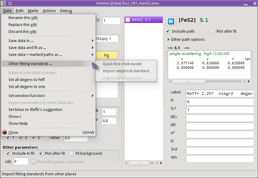
To start, I imported the FeS2 data and crystal structure into ARTEMIS. (You can find them here.) I ran ATOMS, then FEFF. I then dragged and dropped the nearest neighbor path onto the Data page. At this stage, ARTEMIS looks like this:

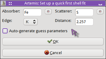
I begin a QFS calculation by selecting that option from the menu on the Data page:

The nearest neighbor path in FeS₂ is a S atom at 2.257 Å.

Clicking OK, the QFS path is generated. I set the degeneracy of the QFS path to 6 so that I can directly compare the normally calculated path (there are 6 nearest neighbor S atoms in FeS₂) to the QFS path. I mark both paths and transfer them to the plotting list. I am now ready to compare these two calculations. To examine another single scattering path, I drag and drop that path from the FEFF page to the Data page and redo the QFS calculation at that distance.