10.2. Principle components analysis
Principle components analysis (PCA) is an abstract decomposition of a data sequence....
Note
This chapter is incomplete.
Here, I have imported a project file containing well-processed data on a time series of samples in which gold chloride is being reduced to gold metal. The project file includes 8 time steps and 9 standards. I cannot stress strongly enough the importance of doing a good job of aligning and normalizing your data before embarking on PCA. This is truly a case of garbage-in/garbage-out.
I then select the PCA tool from the main menu.
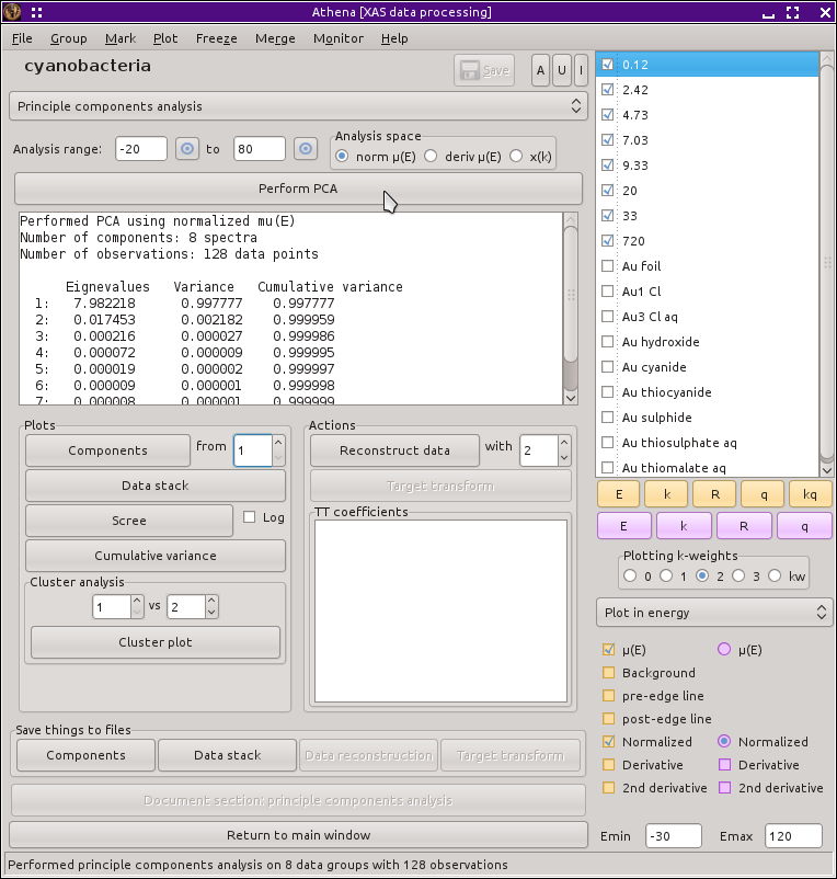
Fig. 10.5 The PCA tool.
The operational concept for the PCA tool makes use of the standard ATHENA group selection tools. The ensemble of marked groups are used as the data on which the PCA will be performed. The selected group (i.e. the one highlighted in the group list) can be either reconstructed or target transformed. The relevant controls will be enabled or disabled depending on whether the selected group is marked (and therefore one of the data sets in the PCA) or not (and therefore a subject for target transformation).
Clicking the Perform PCA button will perform normalization on all the data as needed, then perform the components analysis. Upon completion, some results are printed to the text box and several buttons become enabled.
After the PCA completes, a plot is made of the extracted components. This plot can be recovered by clicking the Components button under the Plots heading. The number spinner is used to restrict which components are plotted. Because the first component is often so much bigger than the rest, it is often useful to set that number to 2, in which case the first (and largest) component is left off the plot.
Other plotting options include a plot of the data stack, as interpolated into the analysis range, a scree plot (i.e. the eigenvalues of the PCA) or its log, and the cumulative variance (i.e. the running sum of the eigenvalues, divided by the size of the eigenvector space). The cluster analysis plot is not yet implemented.
Once the PCA has been performed, you can reconstruct your data using 1 or more of the principle components. Here, for example, is the reconstruction of an intermeidate time point using the top 3 components.
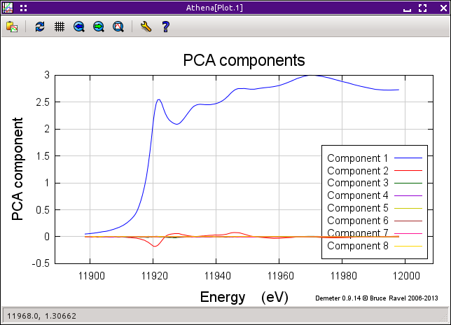
Fig. 10.6 The principle components of this data ensemble.
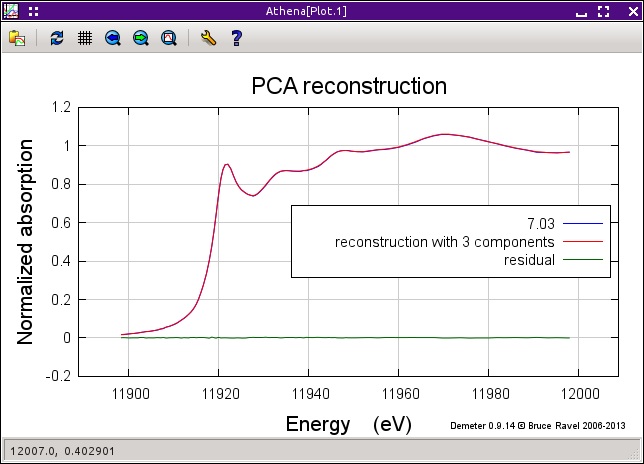
Fig. 10.7 PCA reconstruction
Selecting one of the standards in the group list enables the Target transform button. Clicking it shows the result of the transform and displays the coefficients of the transform in the smaller text box.
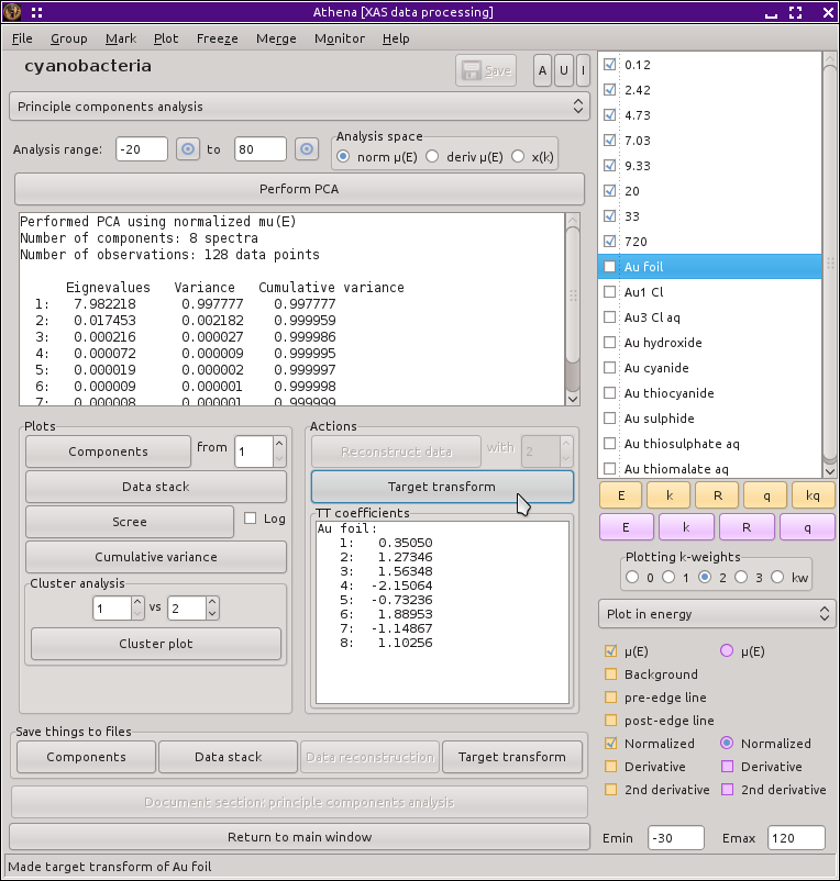
Fig. 10.8 Performing a target transform against a data standard
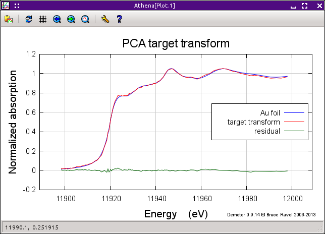
Fig. 10.9 A successful target transform on Au foil. Au foil is certainly a constituent of the data ensemble used in the PCA.
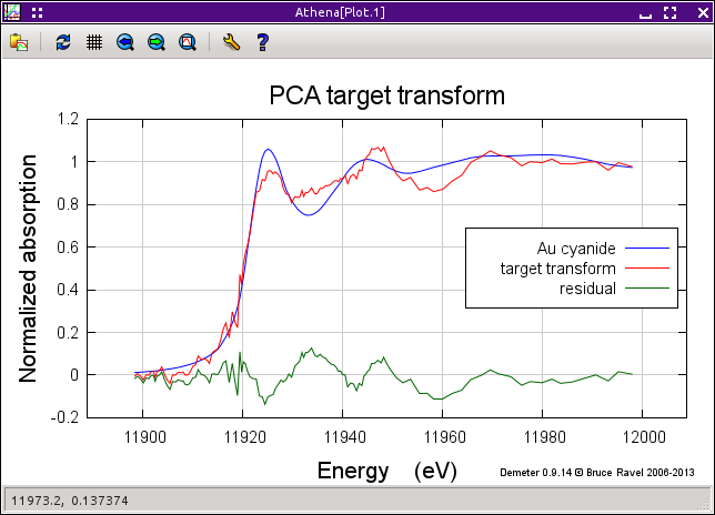
Fig. 10.10 An unsuccessful target transform on Au cyanide. Au cyanide is certainly not a constituent of the data ensemble used in the PCA.
The list of chores still undone for the PCA tool can be found at my Github site.
DEMETER is copyright © 2009-2016 Bruce Ravel – This document is copyright © 2016 Bruce Ravel
This document is licensed under The Creative Commons Attribution-ShareAlike License.
If DEMETER and this document are useful to you, please consider supporting The Creative Commons.