10.3. Peak fitting
10.3.1. Interpreting data as a sum of line shapes
Peak fitting involves fitting a number of analytical line shapes to
XANES data. The typical approach is to simulate the XANES data using
one or two step-like functions and several peak functions for the
peaks in the data. The centroids, amplitudes, and widths of the
various line shapes are either fixed or varied to best fit the
data. In ATHENA's implementation of peak fitting, a
Levenberg-Marquardt non-linear least-squares minimization is used. (To
be specific, IFEFFIT's minimize command is used after
constructing an array with a sum of line shapes or LARCH's
minimize function is using an objective function which contructs
an array with a sum of the line shapes.)
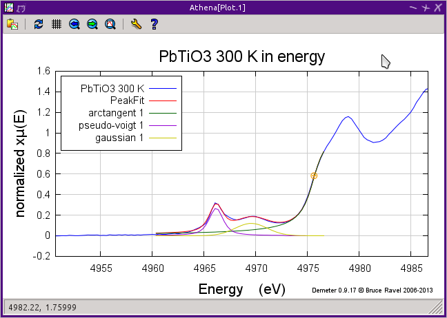
Peak fitting is an inherently empirical analysis technique. By themselves, the line shapes used have little physical meaning. The utility of peak fitting is in quantifying the variation of certain spectral features in a sequence of data. As an example, consider the small peak that appears just before the main rising part of the edge in the perovskite PbTiO3. In the plot below, this is the peak around 4967 eV. This peak varies as a function of temperature as you approach then exceed the crystallographic phase transition. The size of the peak can be related to the amount of displacement of the Ti atom from the near-by postition of centrosymmetry. Peak fitting is a useful tool in this temperature-dependent study as it can quantify the relationship between a spectral feature and an extrinsic parameter.
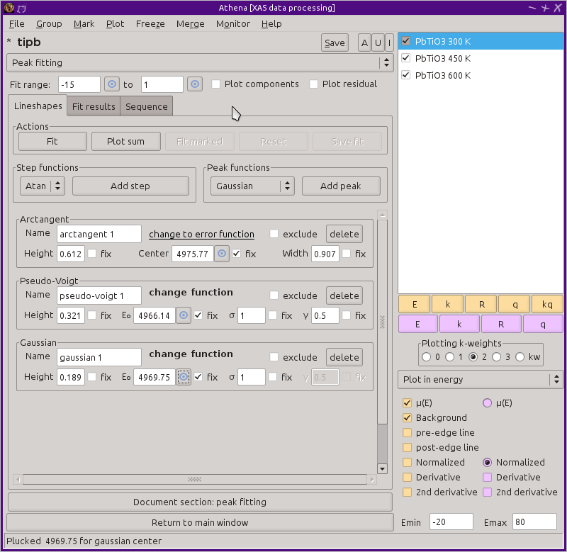
The screenshot above shows the peak fitting tool. The available line shapes when useing IFEFFIT include
- arc tangent (step-like)
- error function (step-like)
- Gaussian (peak)
- Lorentzian (peak)
- pseudo-Voigt (peak)
LARCH adds one step-like function and several peak functions:
- logistic (step-like)
- Voigt (step-like)
- Pearson7 (peak)
- Student's T (peak)
An obviously useful function are not available in the current version of ATHENA is a broadened Cromer-Lieberman calculation of the bare atomic edge step (which might better approximate the shape of the XANES data).
Each line shape has an independent centroid, amplitude, and width. A few line shapes have a fourth parameter. For instance, the pseudo-Voigt function has a parameter for mixing Gaussian and Lorentzian content. By default, the centroids are fixed and the other parameters are varied in the fit.
The peak shapes are unit normalized. This means that the amplitude is the area under the peak.
Here is the result of a fit to the PbTiO3 after slightly tweaking the centroids of the three lineshapes from the values shown above.
10.3.2. Fitting a single data group
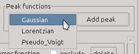
Line shapes are added to the fitting model by clicking the buttons labeled Add step or Add peak. The functional form of the lineshape is chosen by selection from the menu to the left of those buttons.
Clicking one of the Add buttons inserts a field for that lineshape in the area below the buttons. In the screenshot above, three lineshapes have been added: one arc-tangent to model the main edge step, a pseudo-Voigt function to model the first pre-edge peak, and a Gaussian to model the second pre-edge peak.
ATHENA cannot know what feature in the data each line shape is intended to model. You must select the centroid of each line shape. This can be done by typing an energy value into the box labeled either Center or E0. Alternately, you can use the pluck button to take the energy value from the plot using the mouse.
When the pluck button is used, ATHENA will make a guess for the initial value of the height of the lineshape. This is the value of the data at the position plucked for the centroid. The initial guess for the width of the line shape is 0.5 eV for peak shapes and the core-hole lifetime in eV units for the absorbing element of the data being fitted.
Which parameters are fixed and which are varied are controlled by the check buttons labeled Fix next to each parameter value. By default, the centroid is fixed and the other two (or three) parameters are floated in the fit. In my experience, the fits are fairly unstable when the centroids are varied, particularly with peak functions placed close together. I typically leave the centroid values fixed, adjusting them by hand and rerunning the fits if necessary.
The Reset button (which becomes enabled only after a fit is performed) is used to restore parameters for each lineshape to their default values. This is handy if a fit results in strange values due to some numerical instability of the fitting model, which might happen, for example, if centroids are floated.
If you wish to try a different lineshape at the same energy position, you can click on the change function hot text to post a menu of other choices for line shape.
With IFEFFIT, there are only two step-like shapes. So for changing the shape of a step-like function, the hot text simply toggles between the two.
Once you have set all the parameters of the fitting model, the fit is performed by clicking the Fit button in the Actions section at the top of the page. Alternately, you can examine the current state of the model without running the fit by clicking the Plot sum button.
10.3.3. The fit results tab
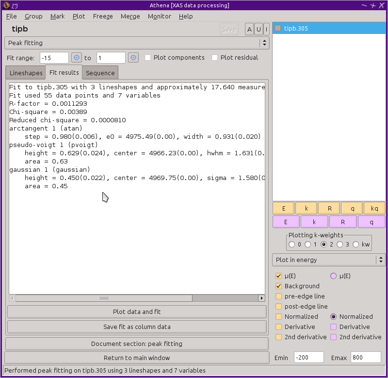
After a fit finishes, the remaining buttons in the Actions section are enabled and the text box on the results tab is filled in with the outcome of the fit.
The Plot data and fit button at the bottom of the results tab makes the same plot as the Plot sum button on the main tab. The plot can be modified to include traces for each individual line shape and for the residual of the fit by toggling the checkbuttons above the note tabs.
The result of the fit can be saved to a column data file by clicking that button at the bottom of the results tab. (The same thing happens with the Save fit button on the main tab.) The output file contains the fit results in the header and has columns of
- energy
- the data
- the fit
- the residual
- one column for each component
10.3.4. Fitting multiple groups and the sequence tab
Once you have found a fitting model that works for a representative data set, ATHENA offers soem automation for examining an ensemble of data. The button on the main tab labeled Fit marked will apply the current fitting model to every marked group in the data list in sequence. For example, in the case of the temperature dependent PbTiO3 data measured at the Ti K edge, we see the first pre-edge peak reduces in size in the measured data as the temperature rises. Consequently, we would expect to see measured height of that peak get smaller with temperature.
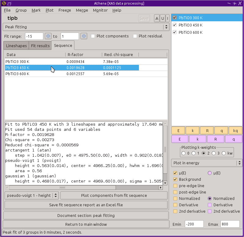
The results of the sequence of fits using the fitting model are shown in the Sequence tab. You can have each fit plotted during the sequence by setting the ♦Peakfit→plot�_during parameter.
The table at the top shows the R-factor and reduced χ2
for each fit in the sequence. Selecting a row of this table by
 clicking on it will display the detailed results
from that fit in the text box and will plot the result of that fit.
ATHENA provides a couple of ways of examining the results of the fit sequence. The list of parameters that were varied in the fit are loaded into the menu just below the text box. Selecting a parameter then clicking on the adjacent plot button will show the evolution of that parameter over the ensemble of data.
Here we see the example of the height of the pseudo-Voigt line shape as a function of temperature. As expected, the value trends downward.
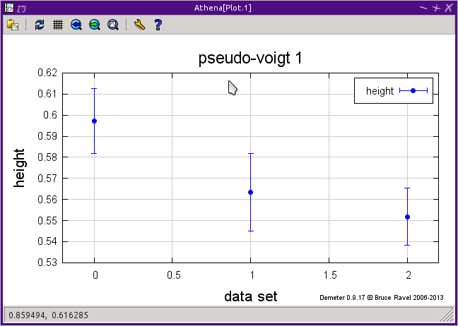
Fig. 10.17 The results for peak height for the feature 4967 eV as measured over the entire data ensemble.
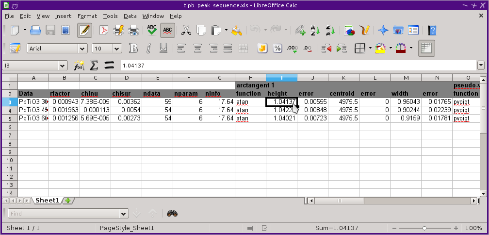
Finally, the results of the fitting sequence can be exported to a spreadsheet file for easy viewing and manipulation in a spreadsheet program, such as Excel, LibreOffice Calc, or Google Docs. This spreadsheet contains the statistics for each fit along with all the parameter values and their uncertainties.
DEMETER is copyright © 2009-2016 Bruce Ravel – This document is copyright © 2016 Bruce Ravel
This document is licensed under The Creative Commons Attribution-ShareAlike License.
If DEMETER and this document are useful to you, please consider supporting The Creative Commons.
