3.1. Column selection dialog
3.1.1. Converting raw data to mu(E)
To import a data file, select or
type Control-o. Alternately, you can
 drag one or more data files from your computer's file
manager and drop them onto the group list. A file selection dialog
opens. On my Linux computer, it looks like this:
It looks somewhat different on Windows, but behaves the same. It allows you to navigate your disk to find the file you want to import. Once you find that file, click on it then click on the Open button.
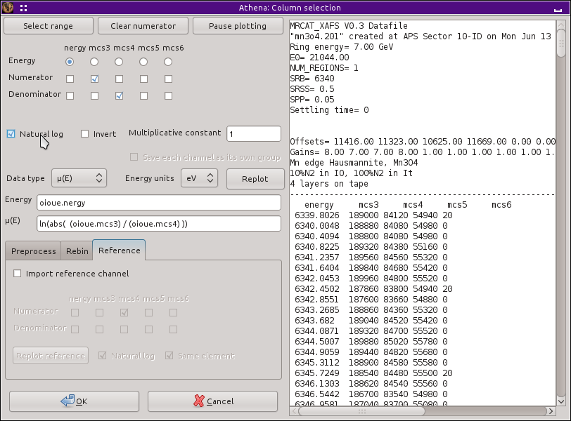
Once you have selected a file to import the column selection dialog, shown below, appears.
On the right side of this dialog, the contents of the data file are displayed. This allows you to examine the file to help you figure out which columns should be imported to turn into the μ(E) data.
On the left are various control for specifying which columns contain the energy values and which contain the signals from the various detectors. Typically, the signals from the detectors are saved to disk as columns of numbers. These columns need to be combined depending on the nature of the experiment. For a transmission experiment, the incident channel is divided by transmission channel and the natural log is taken at each point. For fluorescence data, the fluorescence channel is divided by the incidence channel. Electron yield data is like fluorescence data – the yield channel is divided by the incident channel.
The controls in the tabs at the bottom left are the discussed in later sections.
In the example shown, the incident channel is, for some reason, called mcs3. Since this is transmission data, I have checked the mcs3 button for the numerator. The transmission channel is called mcs4 and its button is checked for the denominator.
As you check the buttons, some helpful things happen. The first is that equation for how the columns combine to form μ(E) is displayed in the box below the column selection buttons. Also as you check buttons, the data are plotted. If you have selected the correct columns and chosen the numerator and denominator correctly, the plot will look like XAS data. If the plot is upside-down, then you need to switch the numerator and denominator. If the plot doesn't look like XAS at all, you need to try some of the other channels.
I chose this example because the columns are labeled somewhat confusingly. Often the columns will be labeled in the file more obviously with names like “I0” or “It”. In this case, we either need to know what the columns mean or patiently click through the buttons to figure it out. As a last resort, you may need to ask the beamline scientist!
3.1.2. Data types and energy units
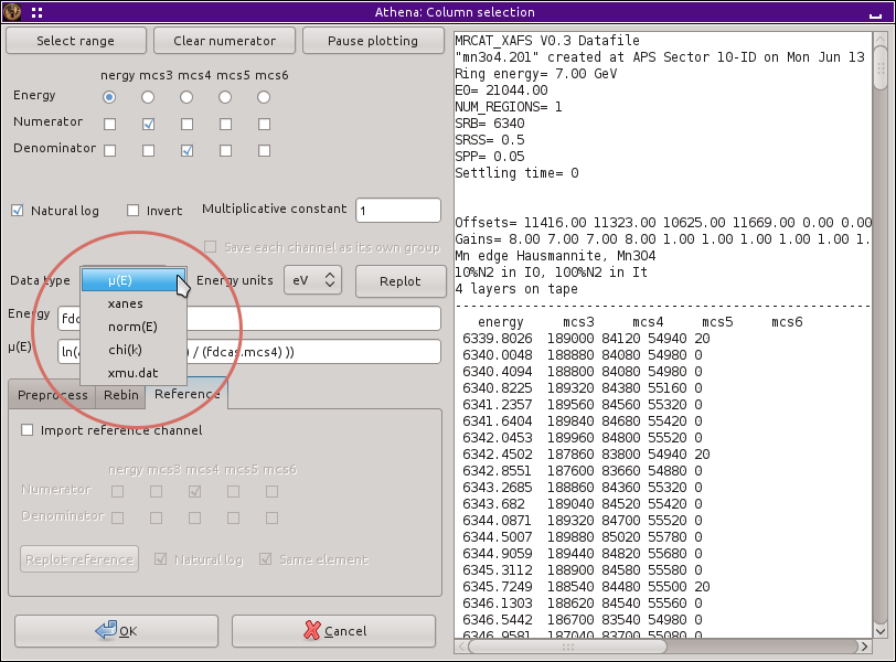
Occasionally, ATHENA needs a bit more information to interpret your data correctly. The data types menu is shown in the figure below. The default is for data to be imported as μ(E).
The other choices are:
- xanes(E) : μ(E) data measured over a limited data range and for which you do not need to look at the χ(k)
- norm(E) : μ(E) data that have already been normalized in some other way. These data will not be normalized by ATHENA
- chi(k) : χ(k) data, that is data that have already been background subtracted from μ(E)
- xmu.dat : the xmu.dat file from FEFF
If you make a mistake and import your data as the wrong data type, you can change between any of the energy-valued (μ(E), normalized μ(E), XANES, or detector) record types at any time by select and selecting the correct choice from the popup dialog, shown here. This dialog cannot, however, be used to change χ(k) data to an energy-value type or vice-versa, nor to change one of the FEFF types to a non-FEFF type.
ATHENA uses electron volts as its energy unit. It uses a simple heuristic to figure out if an input file is in eV or keV. In case ATHENA gets it wrong, you can specify the energy unit with the Energy units menu. Dispersive XAS, i.e. data which is a function of pixel index, requires special treatment.
New in version 0.9.20: There is now a label on the main page right
next to the Freeze check button which identifies the file
type of the data. You can toggle between xanes and xmu data by
Control-Alt- on that label.
3.1.3. Multi-element detector data
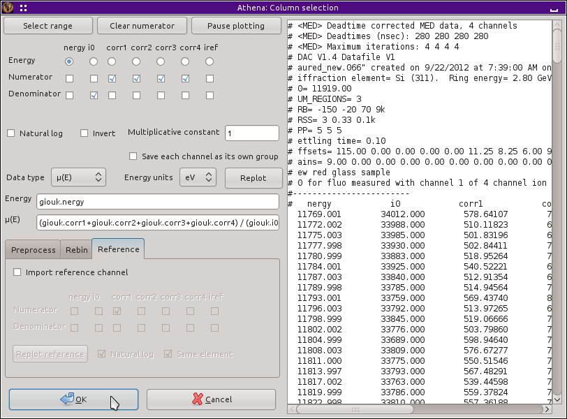
ATHENA's column selection dialog has some special features for dealing with multi-element detectors. You can select all the channels of the MED as elements of the numerator, as shown in this example of the column selection dialog.
Importing the data will then add up the channels on the fly and put a group containing the summation of the channels in the group list.
You have the option of clicking the check button that says Save each channel as its own group, as shown here.
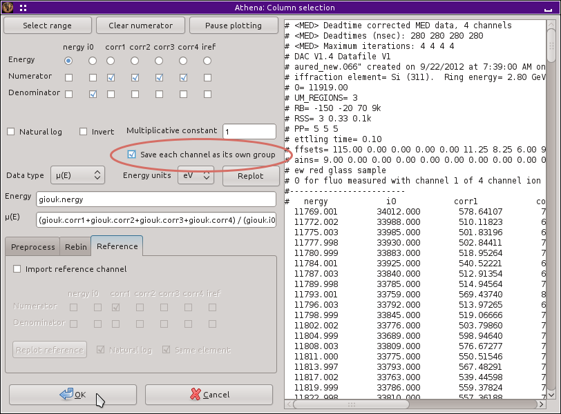
Fig. 3.6 Importing multi-element data in the column selection dialog and saving each channel as a group.
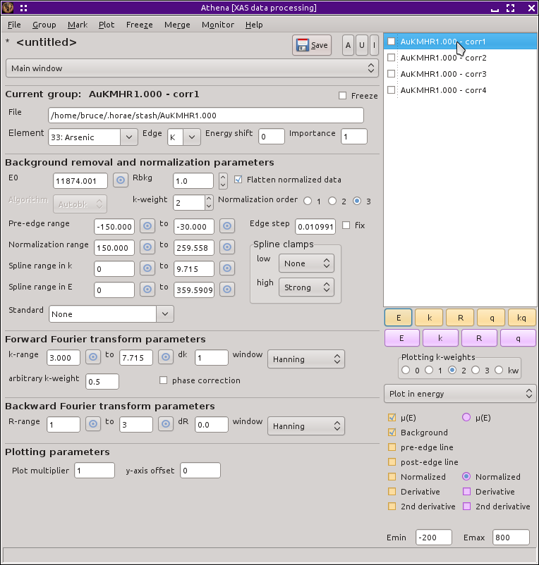
Then, instead of adding the channels to make one group, each channel will be imported as an individual group and given its own entry in the group list. This is handy for examining the channels and discarding any that are not of usable quality.
3.1.4. Other controls
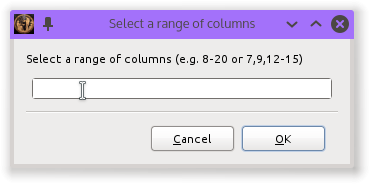
At the top of the page are three buttons for refining how the column selection dialog interacts with your data. The Select range button pops open a dialog which allows you to specify a range of numerator buttons to click all at once.
This expects column numbers not labels. The main purpose of this dialog is to deal with MED data with a large number of columns. It would be tedious and error prone to click through a lot of columns. This dialog is a way of quickly accomplishing that.
You can specify a list of comma-separated column numbers or indicate a range using a dash. In the first example in the text in Fig. 3.8, columns 8 through 20 would be selected. In the second, column 7 and column 9 along with columns 12, 13, 14, and 15 would be selected.
The Clear numerator button unselects all the numerator check button.
The Pause plotting button will suppress the re-display of the plots as you select check buttons in the column selection dialog. This is handy if, for some reason, the re-display of the plot is slow or otherwise undesirable.
DEMETER is copyright © 2009-2016 Bruce Ravel – This document is copyright © 2016 Bruce Ravel
This document is licensed under The Creative Commons Attribution-ShareAlike License.
If DEMETER and this document are useful to you, please consider supporting The Creative Commons.

