9.4. Rebinning data groups
Some beamlines offer the option of slewing the monochromator continuously from the beginning of the scan to the end. A typical implementation of this works by driving the mono at a given speed and reading the measurement channels continuously. The signal is integrated for bins of time. After each time interval, the integrated signals are stored in a buffer. At the end of the scan, the buffer is dumped to disk. When I was at my old beamline (MRCAT, Sector 10 at the APS), a typical EXAFS scan measured in this mode took 3 minutes or less back in those days.
The drawback of this measurement mode (other than the generation of tons of data that needs to be analyzed!) is that the data are vastly over sampled. The energy grid is typically 0.3 to 0.5 eV. That is fine in the edge region, but much too fine for the EXAFS region.
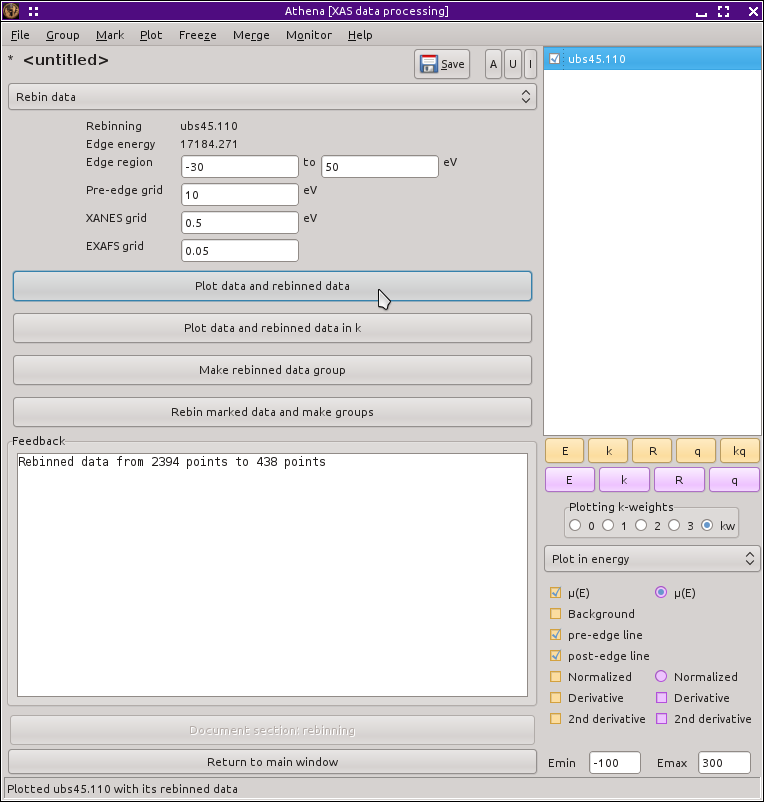
Fig. 9.8 The rebinning tool.
The tool shown above allows you to specify a simple three-region grid. Typically, the pre-edge region is sparse in energy, the edge region is fine in energy, and the EXAFS region is uniform in wavenumber. The grid sizes and the energies of the boundaries are entered into their entry boxes. You can view the results of the rebinning by pressing the Plot data and rebinned data button. The Plot data and rebinned data in k button displays the two spectra as χ(k) using the background removal parameters of the unbinned data. Clicking the Make rebinned data group button performs the rebinning and makes a new group. This group gets placed in the group list and can be interacted with just like any other group.
You can bulk process data by marking a number of groups and clicking the Rebin marked data and make groups button. This may take a while, depending on how many groups are being processed.
This deglitching algorithm is the same as the one used by the rebinning feature of the column selection dialog.
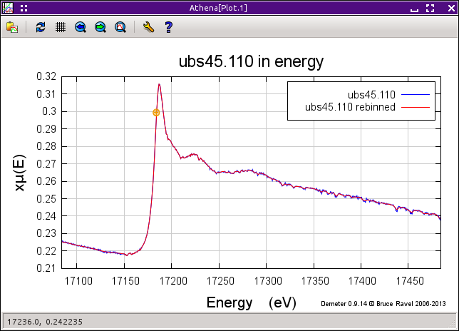
Fig. 9.9 Quick scan data that have been rebinned onto a normal EXAFS energy grid.
This uses a boxcar averaging to put the measured data on the chosen grid. This has the happy effect of cleaning up fairly noisy data, as you can see in the plot above.
DEMETER is copyright © 2009-2016 Bruce Ravel – This document is copyright © 2016 Bruce Ravel
This document is licensed under The Creative Commons Attribution-ShareAlike License.
If DEMETER and this document are useful to you, please consider supporting The Creative Commons.