13.1. Example 1: FeS2

Iron pyrite, FeS₂, is my favorite teaching example which I use to introduce people to fitting with ARTEMIS. It is a crystal with a well-known structure. I have beautiful data. And I am able to create a very successful fitting model. As a cubic crystal, the structure is not too complicated. However, there is some internal structure in the unit cell, making this a much less trivial example than, say, an FCC metal.

While this example certainly does not represent a typical research problem, it is an excellent introduction to the mechanics of using ARTEMIS and it results in a very satisfying fit.

You can find example EXAFS data and crystallographic input data at my XAS Education site. Import the μ(E) data into ATHENA. When you are content with the processing of the data, save an ATHENA project file and dive into this example.

13.1.1. Import data

After starting ARTEMIS, click on the Add button at the top of the Data sets list in the Main window. This will open a file selection dialog. Click to find the ATHENA project file containing the data you want to analyze. Opening that project file displays the project selection dialog.

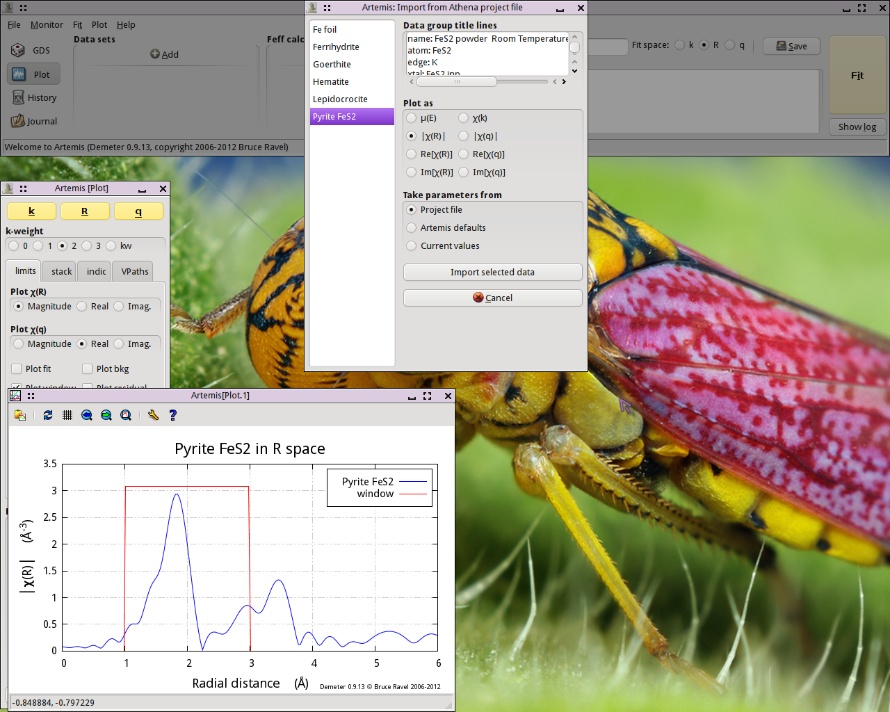
Fig. 13.1 Import data into ARTEMIS

The project file used here has several iron standards. Select FeS₂ from the list. That data set gets plotted when selected.

Now click the Import button. That data set gets imported into ARTEMIS. An entry for the FeS₂ is created in the Data list, a window for interacting with the FeS₂ data is created, and the FeS₂ data are plotted as χ(k).

The next step is to prepare for the FEFF calculation using the known FeS₂ crystal structure. Clicking on the line in the Data window that says Import crystal data or a Feff calculation will post a file selection dialog. Click to find the atoms.inp file containing the FeS₂ crystal structure.

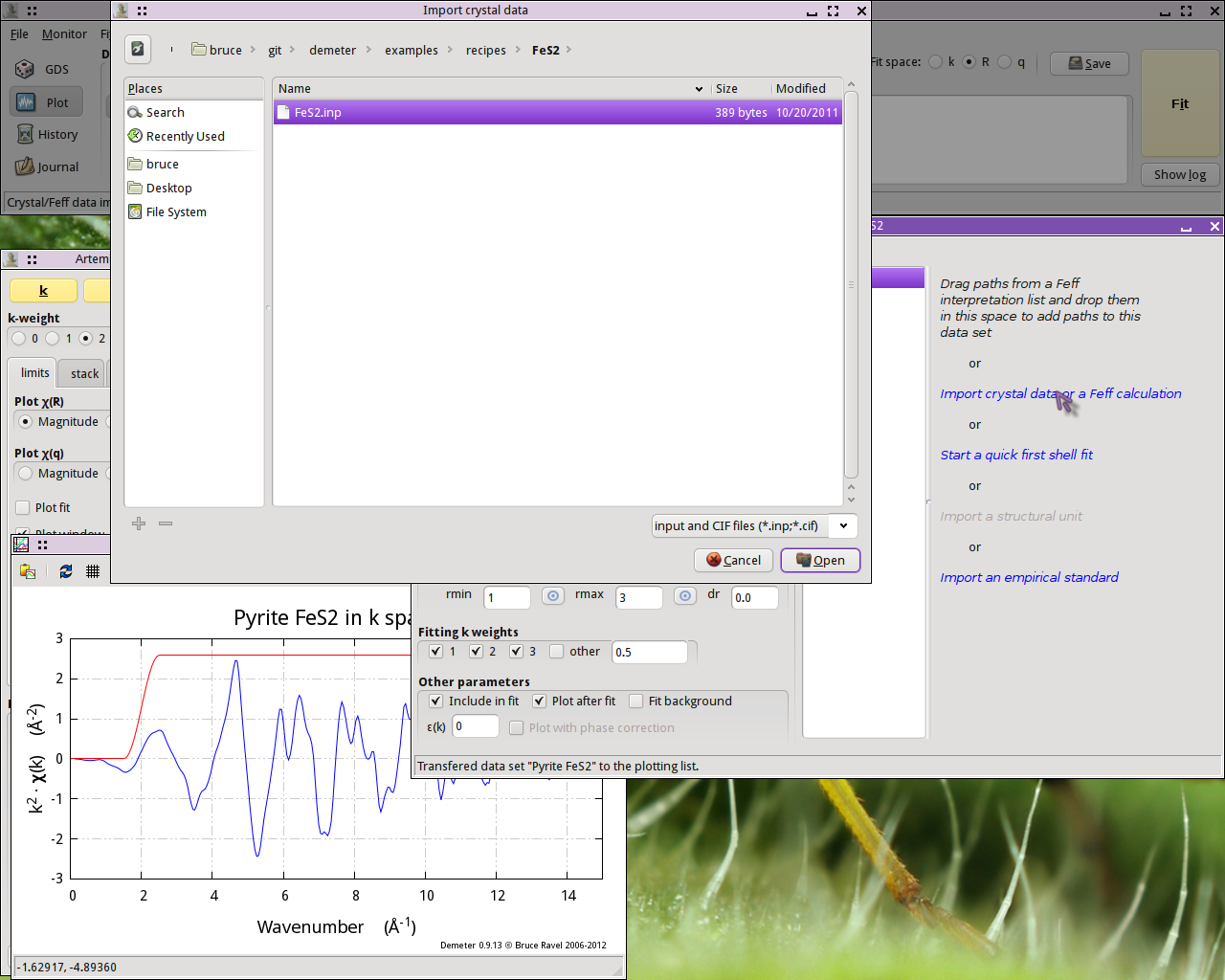
Fig. 13.2 Import crystal data into ARTEMIS

With the FeS₂ crystal data imported, run ATOMS by clicking the Run Atoms button on the ATOMS tab of the FEFF windows. That will display the FEFF tab containing the FEFF input data. Click the Run Feff button to compute the scattering potentials and to run the pathfinder.

Once the FEFF calculation is finished, the path intepretation list is shown in the Paths tab. This is the list of scattering paths, sorted by increasing path length. Select the first 11 paths by clicking on the path 0000, then Shift- clicking on path 0010. The selected paths will be highlighted. Click on one of the highlighted paths and, without letting go of the mouse button, drag the paths over to the Data window and drop them onto the empty Path list.

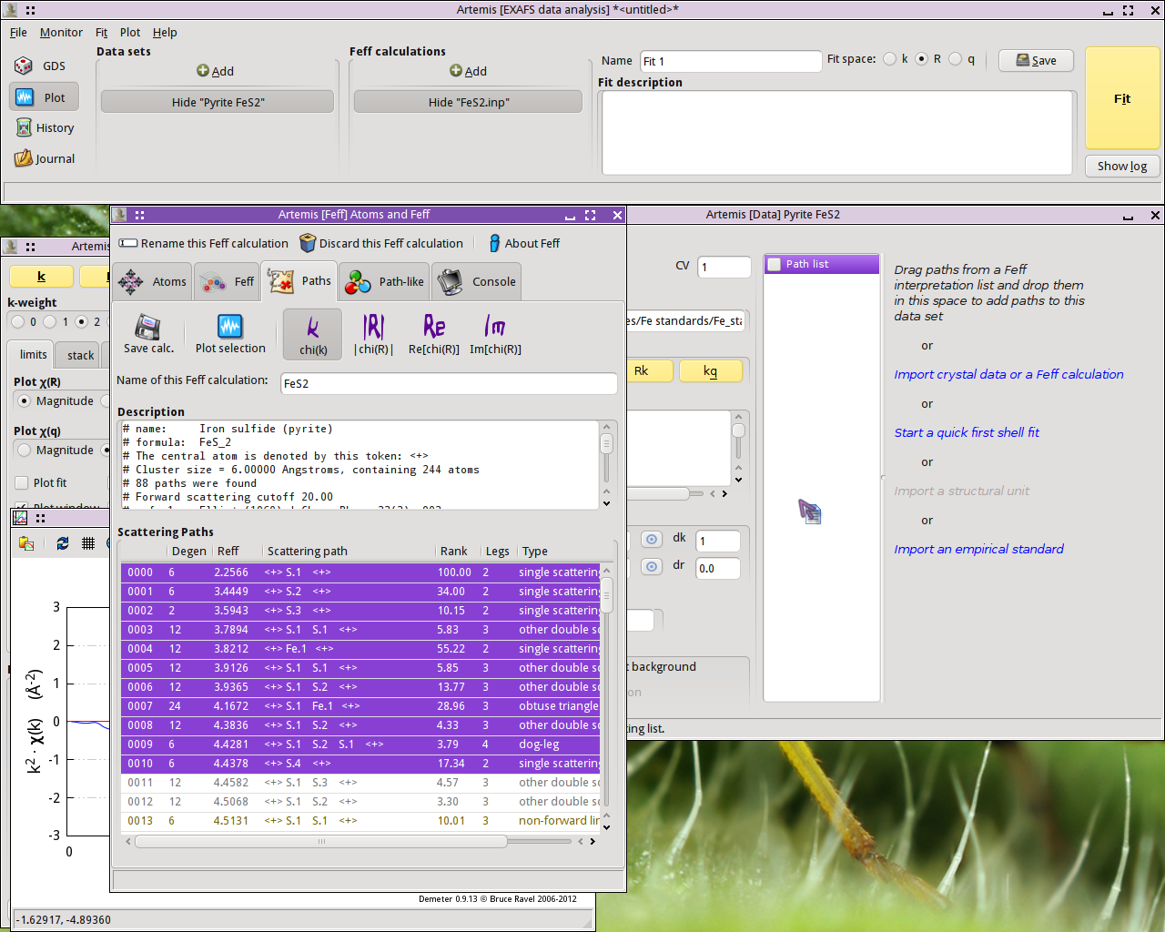
Fig. 13.3 Drag and drop paths onto a data set

Dropping the paths on the Path list will associate those paths with that data set. That is, that group of paths is now available to be used in the fitting model for understanding the FeS₂ data.

Each path will get its own Path page. The Path page for a path is displayed when that path is clicked upon in the Path list. Shown below is the FeS₂ data with its 11 paths. The first path in the list, the one representing the contribution to the EXAFS from the S single scattering path at 2.257 Å, is currently displayed.

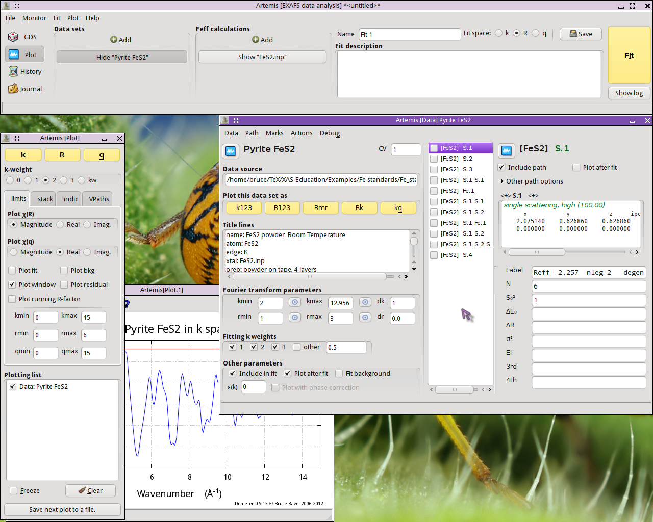
Fig. 13.4 Paths associated with a data set

13.1.2. Examine the scattering paths

The first chore is to understand how the various paths from the FEFF calculation relate to the data. To this end, we need to populate the Plotting list with data and paths and make some plots.

First let's examine how the single scattering paths relate to the data. Mark each of the first four single scattring paths – the ones labeled S.1, S.2, S.3, and Fe.1 – by clicking on their check buttons. Transfer those four paths to the Plotting list by selecting Actions ‣ Transfer marked.

With the Plotting list poluated as shown below, click on the R plot button in the Plot window to make the plot shown.

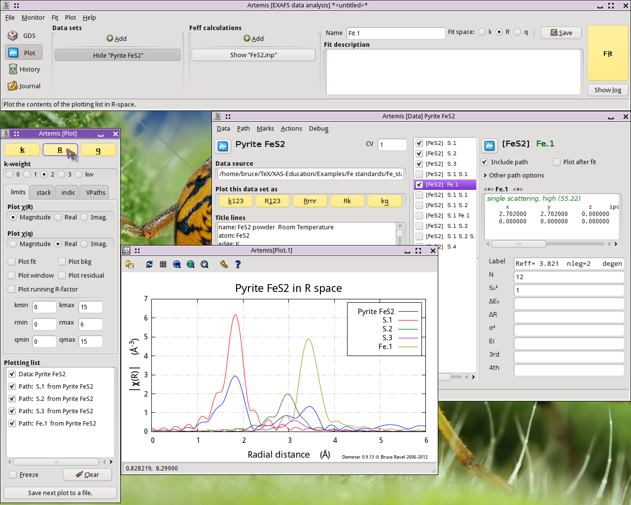
Fig. 13.5 FeS₂ data plotted with the first four single scattering paths

The first interesting thing to note is that the first peak in the data seems to be entirely explained by the path from the S atom at 2.257 Å. None of the other single scattering paths contribute significantly to the region of R-space.

The second interesting thing to note is that the next three single scattering paths are not so well separated from one another. While it may be tempting to point at the peaks at 2.93 Å and 3.45 Å and assert that they are due to the second shell S and the fourth shell Fe, it is already clear that the situation is more complicated. Those three single scattering paths overlap one another. Each contriobutes at least some spectral weight to both of the peaks at 2.93 Å and 3.45 Å.

The first peak shold be reather simple to interpret, but higher shells are some kind of superposition of many paths.

What about the multiple scattering paths?

To examine those, first clear the Plotting list by clicking the Clear button at the bottom of the Plot window. Transfer the FeS₂ data back to the Plotting list by clicking its transfer button: . Mark the first three multiple scattering paths by clicking their mark buttons. Select Actions ‣ Transfer marked.

With the Plotting list newly populated, make a new plot of | χ(R)|.

Fig. 13.6 FeS2 data plotted with the first three multiple scattering paths

The two paths labeled S.1 S.1, which represent two different ways for the photoelectron to scatter from a S atom in the first coordination shell then scatter from another S atom in the first coordination shell, contribute rather little spectra weight. Given their small size, it seems possible that we may be able to ignore those paths when we analyze our FeS₂ data.

The S.1 S.2 path, which first scatters from a S in the first coordination shell then from a S in the second coordination shell, contributes significantly to the peak at 2.93 Å. It seems unlikely that we will be able to ignore that path.

To examine the next three multiple scattering paths, clear the Plotting list, mark those paths, and repopulate the Plotting list.

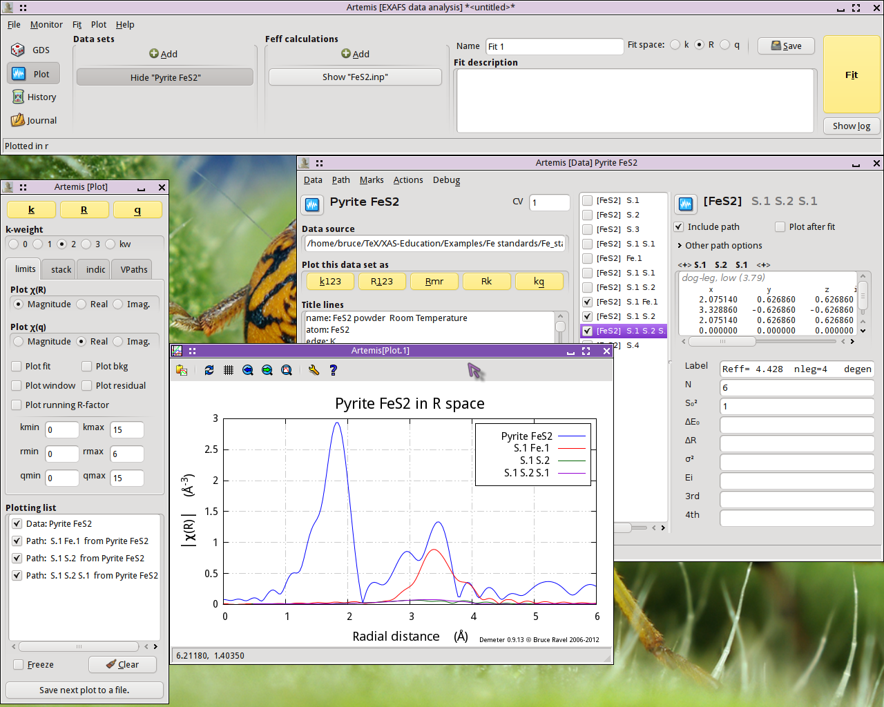
Fig. 13.7 FeS2 data plotted with the next three multiple scattering paths

The S.1 Fe.1 path, which scatters from a S atom in the first coordination shell then scatters from an Fe atom in the fourth coordination shell, is quite substantial. It will certainly need to be considered in our fit. The other two paths are tiny.

13.1.3. Fit to the first coordination shell

We begin by doing an analysis of the first shell. As we saw above, we only need the first path in the path list. To prepare for the fit, we do the following:

1. Exclude all but the first path from the fit. With the first path selected in the path list and displayed, select Marks ‣ Mark after current. This will mark all paths except for the first one. Then select Actions ‣ Exclude marked. This will exclude those paths from the fit. That is indicated by the triple parentheses in the path list.
2. Set the values of R_min and R_max to cover just the first peak.
3. For this simple first shell fit, we set up a simple, four-parameter model. The parameters amp, enot, delr, and ss are defined in the GDS window and given sensible initial guess values.
4. The path parameters for the first shell path are set. S²₀ is set to amp, E₀ is set to enot, ΔR is set to delr, and σ² is set to ss.

Note that the current settings for k- and R-range result in a bit more than 7 independent points, as approximated using the Nyquist criterion. With only 4 guess parameters, this should be a reasonable fitting model.

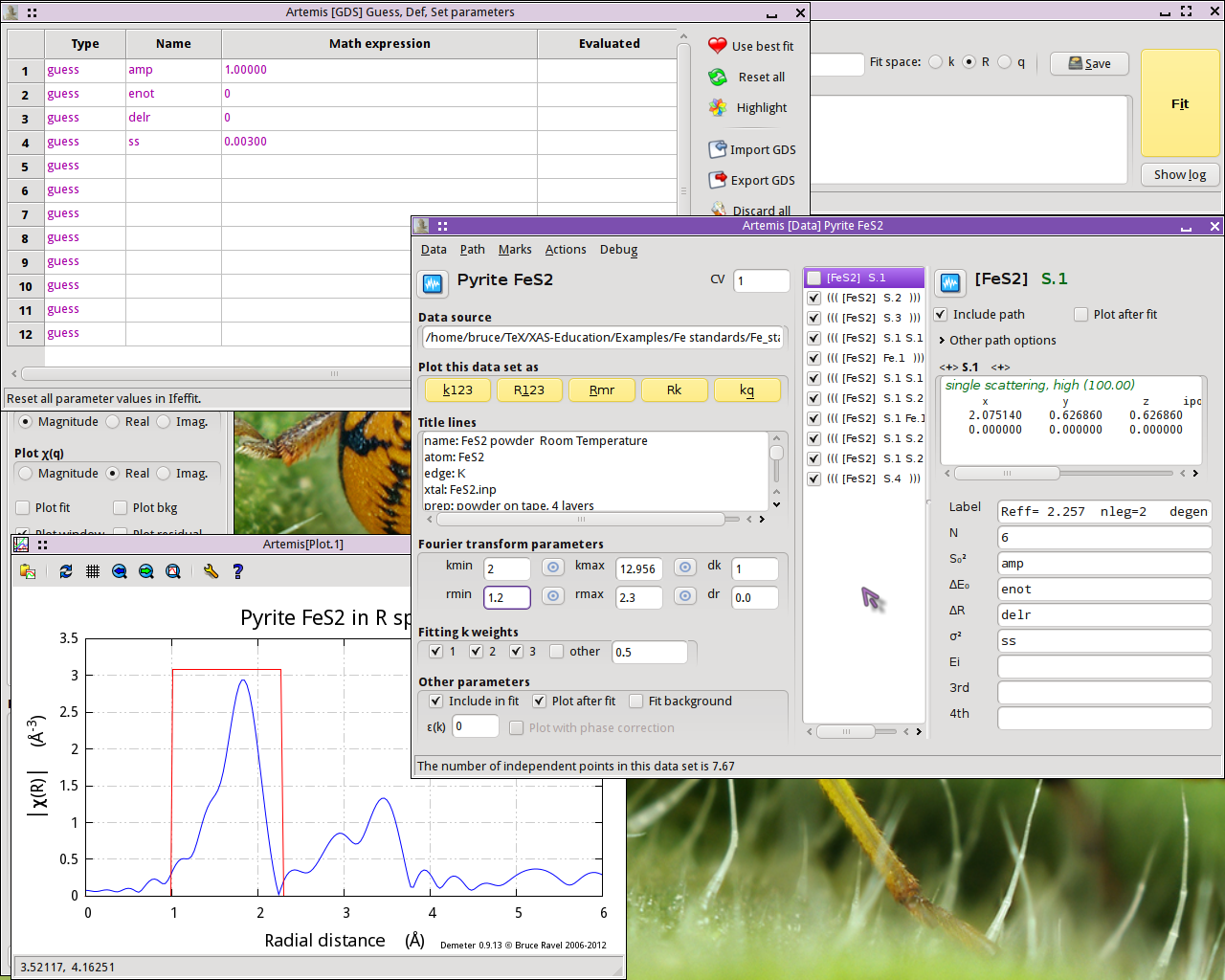
Fig. 13.8 Setting up for a first shell fit

Now hit the Fit button. Upon completion of the fit, the following things happen:

1. An “Rmr” plot is made of the data and the fit.
2. The log Window is displayed with the results of the fit
3. The Fit and plot buttons are recolored according to the evaluation of the happiness parameter.
4. The Plotting list is cleared and repopulated with the data.
5. The fit is entered into the History window (which is not in the screenshot below).

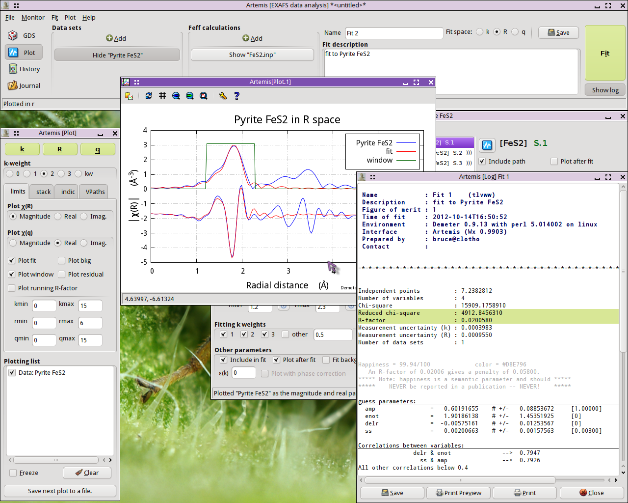
Fig. 13.9 Results of the first shell fit

This is not a bad result. The value of enot is small, indicating that a reasonable value of E₀ was chosen back in ATHENA. delr is small and consistent with 0, as we should expect for a known crystal. ss is a reasonable value with a reasonable error bar. The only confusing parameter is amp, which is a bit smaller than we might expect for a S²₀ value.

The correlations between parameters are of a size that we expect. The R-factor evaluates to about 2% misfit. χ²_v is really huge, but that likely means that ε was not evaluated correctly. All in all, this is a reasonable fit.

13.1.4. Extending the fit to higher shells

Although we know that we will need to include some multiple scattering paths in this fit, we'll start by including the next three single scattering paths, adjusting the fitting model accordingly.

This fit will include the peaks in the range of 3 Å to 3.5 Å, so set R_max to 3.8. Next click on each of next three single scattering paths – the ones labeled S.2, S.3, and Fe.1, then click on the Include path button for each path.

At this point we need to begin considering the details of our fitting model more carefully. S²₀ and E₀ should be the same for each path, so we will use the same guess parameters for each path.

This is a cubic material. Ignoring the possibility that fractional coordinate of the S atom in the original crystal data might be a variable in the fit and considering only the prospect of a volumetric lattice expansion, we define a guess parameter alpha and set the ΔR for each path to alpha*reff.

Finally, we set independent σ² parameters for each single scattering path. This gives a total of 7 guess parameters, compared to the Nyquist evaluation of about 16.5, given the new value of R_max.

Things now look like this:

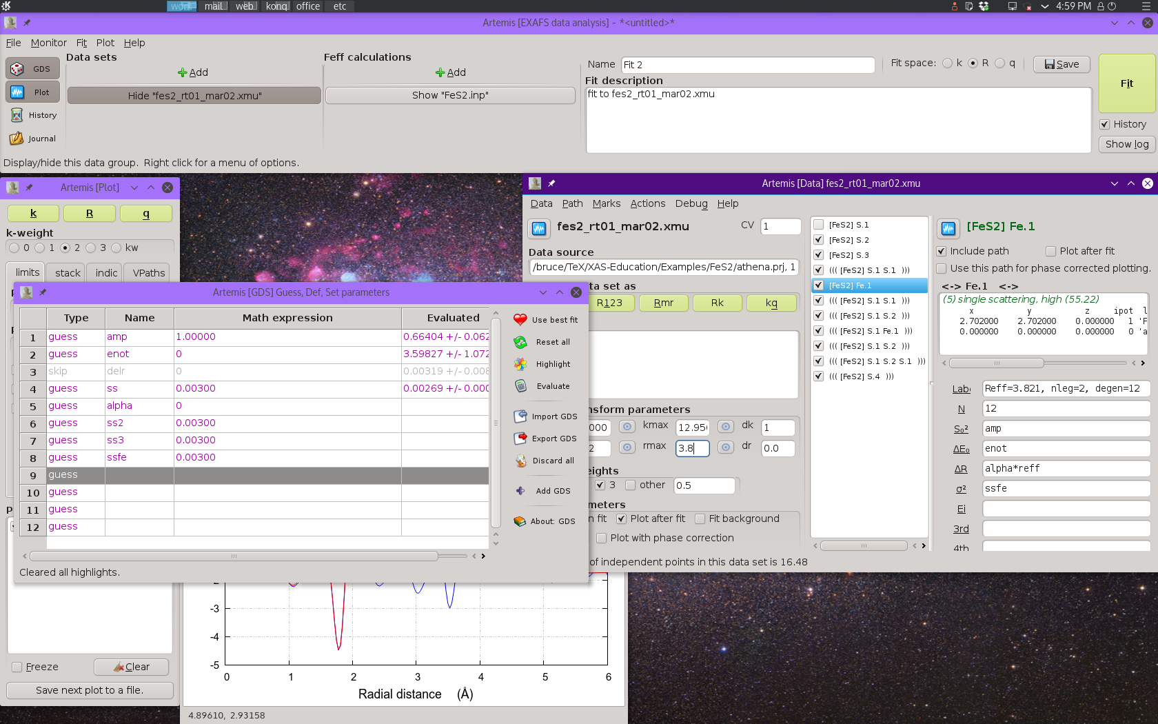
Fig. 13.10 Preparing to run the four-shell fit with only single scattering paths.

At this point we can run the fit and see how things go!

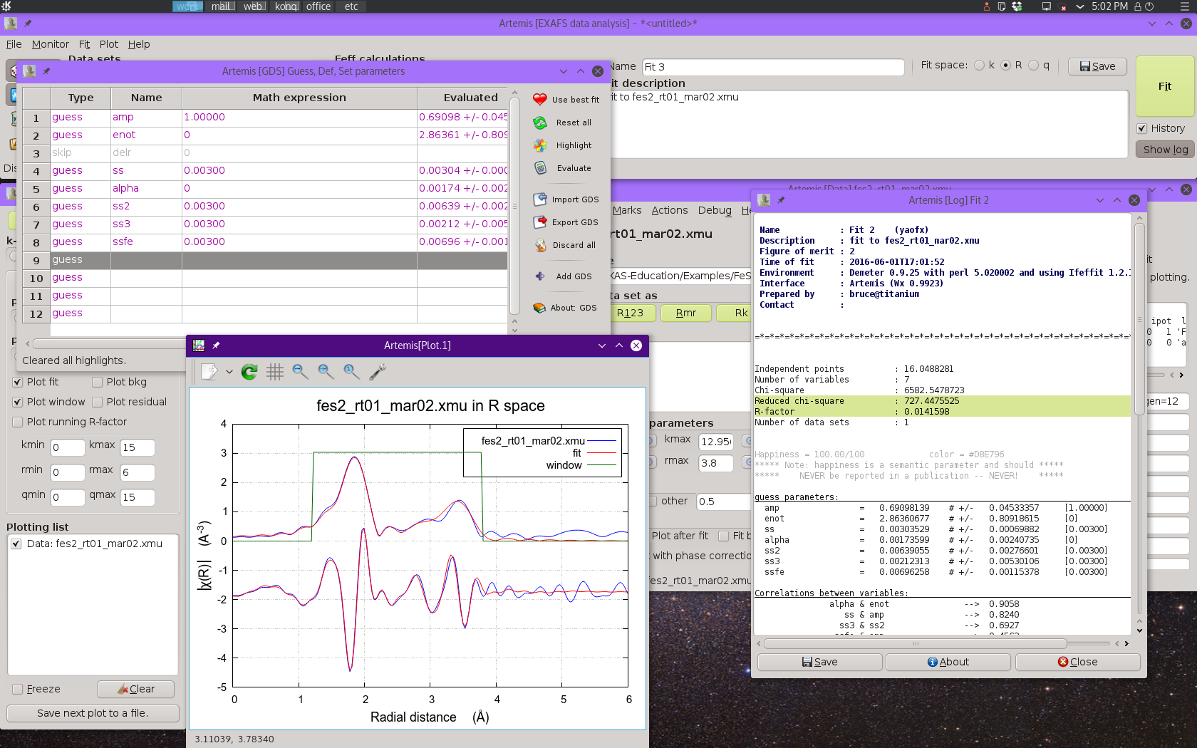
Fig. 13.11 Result of the four-shell fit using on the single scattering paths. Note the misfit around 3.2 Å.

This fit isn't bad. It does a good job of representing the data, with the exception of some misfit around 3.2 Å. Most of the fitting parameters are pretty reasonable, with the exception of the result for ss3. This is discussed in some detail in the lecture notes, but the bottom line is that the signal from these two S scatterers, while a significant contributor of Fourier components to the fit, is not large enough to support its own robust σ² parameter. We will make ss3 into a def parameters, setting it equal to ss2.

Fig. 13.12 Making ss3 a def parameter.

At this point we need to introduce the two significant multiple scattering paths. Start by clicking the Include path button for the S.1 S.2 and S.1 Fe.1 paths.

Make sure each of those paths has their S²₀, E₀, and ΔR path parameters set to amp, enot, and alpha*reff, respectively.

As discussed in the lecture notes, we don't necessarily want to give these multiple scattering paths independent σ² parameters. Indeed, they are unlikely to be robust fitting parameters for the same reason that ss3 proved not to be a robust parameter. Instead, we will approximate these two σ² parameters using guess parameters already in the fit.

Consider these two triangular paths on a leg-by-leg basis. For the S.1 Fe.1 path, the first and last leg are of the distance between the absorber and the Fe scatterer in the fourth shell. The remaining leg is the first shell distance. In terms of length, this path covers the full distance of the fourth shell path and half the distance of the first shell path. Thus we will approximate its σ² as ssfe+ss/2.

The S.1 S.2 triangle is a bit more ambiguous, since we do not have a parameter describing the leg that goes from the first shell S atom to the second shell S atom. In the absence of a better approximation, we will use ss*1.5, i.e. something a bit bigger than the first shell σ². Neither of these are quite right, but neither is ridiculously wrong. And parameterizing them in this way allows us to avoid introducing a weak guess parameter into the fitting model.

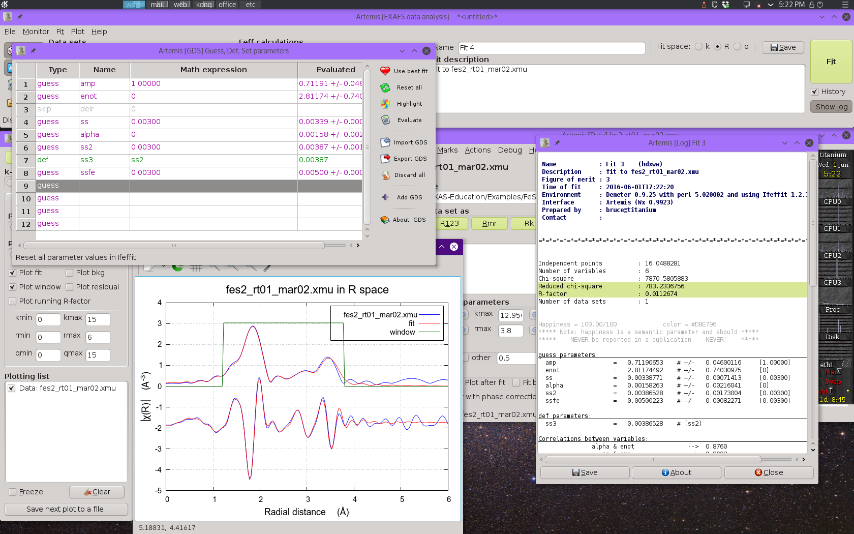
Fig. 13.13 Result of the four-shell fit including four single scattering paths and the two largest multiple scattering paths.

This fit does a much better job in the region around 3.2 Å, however the last bit of the fitting range is not quite right. The fitting parameters are all quite reasonable and the percentage misfit within the fitting range is quite small – around 1%.

13.1.5. The final fitting model

To clean up the last bit of the fitting range, we can include a set of three multiple scattering paths that represent collinear paths involving the first shell S atoms. An ARTEMIS project file for the final fitting model can be found among the examples at my XAS Education site. Adding these three paths and extending R_max to 4.2 Å results in an excellent fit.

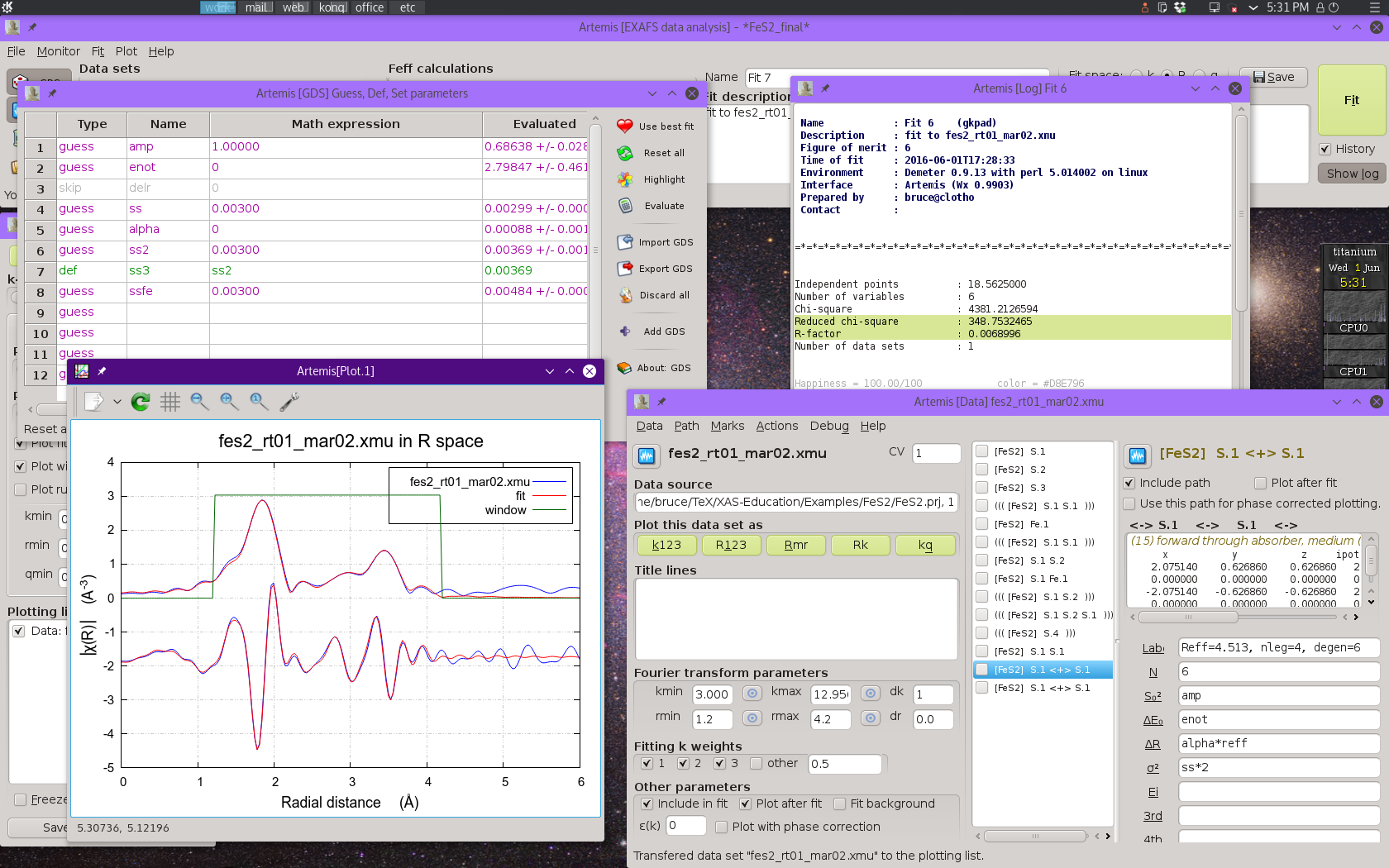
Fig. 13.14 Result of the final fitting model including four single scattering paths and five multiple scattering paths.

These three collinear multiple scattering paths are introduced into the fit without needing to introduce new guess parameters. The alpha*reff parameterization for ΔR works just as well for these paths. Their σ² parameters are expressed in terms of the first shell σ² following the example of Hudson, et al.

• E. A. Hudson, P. G. Allen, L. J. Terminello, M. A. Denecke, and T. Reich. Polarized x-ray-absorption spectroscopy of the uranyl ion: comparison of experiment and theory. Phys. Rev. B, 54:156–165, Jul 1996. doi:10.1103/PhysRevB.54.156.

Please review the lecture notes for this fitting example for discussions of all the decisions that went into creating this successful fitting model.

---

DEMETER is copyright © 2009-2016 Bruce Ravel – This document is copyright © 2016 Bruce Ravel

This document is licensed under The Creative Commons Attribution-ShareAlike License.

If DEMETER and this document are useful to you, please consider supporting The Creative Commons.