15.4. Modeling disorder
The σ2 term in the EXAFS equation accounts for the mean square variation in path length. This variation can be due to thermal or structural disorder. Even in a well-ordered material, like Cu or another FCC metal, data are measured at finite temperature. The absorber and scatterer are both in motion due to the finite temperature. Each interaction of the incident X-ray and the absorber is like a femtosecond snapshot of the coordination environment. As those snapshots are averaged in the EXAFS measurement, σ2 is non-zero, even in the well-ordered material.
A structural disordered contributes another term to σ2. Due to structural disorder, the scatterers which are nominally contained in a scattering shell may be centered around somehwat different distances. When the contributions from those scatterers are considered, σ2 will be larger than what is expected from purely thermal effects.
Consequently, σ2 is always non-zero in an EXAFS fit and a proper interpretation of the fitted value of σ2 will take into account both the thermal and structural component.
It is usually a challenge to distinguish the thermal and structural contributions to σ2. As with any highly correlated effects, the only way to disentangle the two contributions is to do something in the experiment which is sensitive to one or both.
One common approach for understanding the thermal part of σ2 is to measure the sample at two or more temperatures. Assuming the material does not change phase in that temperature range, we expect the thermal part of σ2 to have a temperature dependence while the structural part may reman fixed (or at least change much less). Another possible way to disentangle the two contributions is to measure EXAFS data as a function of pressure. In that case the thermal contribution can be modeled as a function of pressure and a Grüneisen parameter.
15.4.1. Debye and Einstein models
IFEFFIT provides two bult-in functions for modeling σ2 as a function of temperature.
- Einstein model
The Einstein model assumes that the absorber and scatter are balls connected by a quantum spring. They oscillate with a single frequency and the low-temperature motion saturates to a zero-point motion. The function for computing σ2 from the Einstein is a function of the measurement temperature, an Einstein temperature, and the reduced mass of the absorber/scatterer pair. In ARTEMIS one writes:
path:
    sigma2 = eins(temperature, thetae)
Typically,
temepratureis a set parameter whise value is the mesurement tempreature of the data andthetaeis a guess parameter representing the Einstein temprature – i.e. the characteristic frequency of vibration expressed in temeprature units – of the absorber-scatterer pair. The reduced mass is computed by IFEFFIT from the information provided by FEFF about the scattering path.The Einstein function is most useful as part of a multiple data set fit. In that case, a path can have its σ2 parametrized using the
einsfunction and a single ϴE guess parameter is used for all temperatures.When using IFEFFIT, the Einstein function is called
eins(). When using LARCH, it is calledsigma2_eins(). The user of ARTEMIS can use either form with either backend and the correct thing will happen.- Correlated Debye model
The correlated Debye model assumes that the σ2 for any pair of atoms can be computed from the acoustic phonon spectrum. That is, a single charcteristic energy – the same Debye temperature, , that is determined from the heat capacity of the material – can be used to compute σ2 for any path in the material. In ARTEMIS one writes:
path:
    sigma2 = debye(temperature, thetae)
This is a very powerful concept. All σ2 parameters in the fit are determined from a single variable ϴD. The caveat is that the correlated Debye model is only strictly valid for a monoatomic material. In practice, the Debye model works well for metals like Cu, Au, and Pt. It works poorly for any material that has two or more atomic species.
When using IFEFFIT, the Debye function is called
debye(). When using LARCH, it is calledsigma2_debye(). The user of ARTEMIS can use either form with either backend and the correct thing will happen.
Both models are described in
- E. Sevillano, H. Meuth, and J. J. Rehr. Extended x-ray absorption fine structure Debye-Waller factors. I. Monatomic crystals. Phys. Rev. B, 20:4908–4911, Dec 1979. doi:10.1103/PhysRevB.20.4908.
15.4.2. Colinear multiple scattering paths
This valuable paper explains the relationships between σ2 parameters for single scattering paths and certain multiple scattering paths:
- E. A. Hudson, P. G. Allen, L. J. Terminello, M. A. Denecke, and T. Reich. Polarized x-ray-absorption spectroscopy of the uranyl ion: comparison of experiment and theory. Phys. Rev. B, 54:156–165, Jul 1996. doi:10.1103/PhysRevB.54.156.
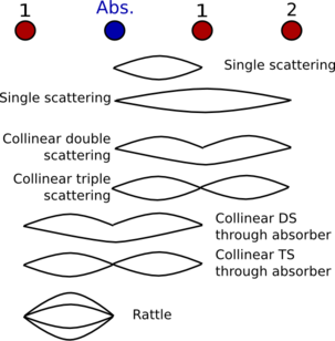
Fig. 15.15 This diagram demonstrates the various kinds of collinear MS paths and how they relate to the corresponding SS path.
To begin, we define guess parameters for the σ2 of the SS paths to atoms 1 and 2.
guess  ss1 = 0.003
guess  ss2 = 0.003
The next two paths are double and triple scattering paths that scatter
in the forward direction from atom 1, then in the backward direction
atom 2. As explained by Hudson, et al., these paths have the same
σ2 as the SS path to atom 2, i.e. σ2 =
ss2 for both these paths.
The next three paths involve scattering from the absorber. The
collinear DS and TS paths simply have σ2 =
2*ss1. The path in which the photoelectron rattles back and forth
between the absorber and atom 1 has σ2 = 4*ss1.
The caveat to these relationships is that the motion of the intervening atom in the perpendicular direction is presumed to be a negligible contribution to the mean square variation in path length. This is, of course, not strictly true. In very high quality data, you may see deviations from the expressions presented by Hudson, et al., but in most cases they are an excellent approximation and a powerful constraint that you can apply to the paths in your fit.
15.4.3. Sensible approximations for triangular multiple scattering paths
In the FeS2 example, we saw that a couple of non-collinear multiple scattering paths contributed significantly to the EXAFS. For these triangular paths, unlike for collinear paths, there is no obvious relationship between their σ2 parameters and the σ2 for the SS paths.
One of the triangular paths in the FeS2 fit was of the form Abs-Fe-S-Abs. The S-Abs leg is like half the first neighbor path. The Fe-S is also like half the first neighbor path. The mean square vairation in path length along those two legs of the path is the σ2 for the first path. Finally, the Abs-Fe leg is like half the fourth shell path.
The math epression for the σ2 of this triangle path was set as
path Fe-S triangle:
    sigma2 = ss1 + ss_fe/2
This approximation of σ2 has the great virtue of not introducing a new parameter to the fit. It neglects any attenuation to the path due to thermal variation in sattering angle. While that is an important effect, there is no simple and accurate way to model it.
This example demonstrates the decision that must be made every time a non-colinear multiple scattering path is considered for a fitting model. In short, you have three choices:
- Do nothing, leave the MS path out of the fit.
- Include the MS path, but allow it to have it's own σ2 parameter.
- Include the MS path, but approximate it's σ2 in terms of parameters which are already part of the fitting model, presumably the parameters of the SS σ2 values.
The Abs-Fe-S-Abs path in FeS2 was really quite large. Going for choice number 1 and leaving it out of the fit is clearly a poor choice.
Number 2 is, in principle, the best choice. As an independently floated parameter, it's σ2 will account for the mean square vriation in path length and the effect of variation in the scattering angle. Unfortunately, this parameter is likely not to be highly robust because it is only used for this one path. There just is not much information available to determine its proper value. And if the fit includes several triangle paths, each of which has a σ2 parameter of similarly weak robustness, the problem becomes amplified.
In almost all cases, option number 3 is the best choice. The approximation is not horribly wrong, thus it introduces only a little bit of systematic error into the fitting model. Including the Fourier components from the path is better than neglecting the path. Since a reasonable approximation can be made without introducing new variable parameters to the fit, the triangle path should be included.
The Abs-Fe-S-Abs path had the virtue that all of its legs were represented by SS paths already included in the fit. Another triangle path was included: Abs-S-S-Abs. In this case, the first and last legs are related to the first coordination shell. The middle leg, S-S, has no corresponding SS path. In the FeS2 example, this triangle path was given a σ2 math expression of 1.5 times the first shell σ2.
This is obviously not accurate. Like all such triangle paths, the decision outlined above must be worked through. In this case, the fit benefits by including this triangle path, but it does not merit having its own floating parameter. I assert that value of σ2 that is “a bit more than the first shell” is reasonable.
This is discussed in more detail in Scott Calvin's book,
- Scott Calvin. XAFS for Everyone. CRC Press, Boca Raton, 2013. ISBN 1439878633. URL: https://www.crcpress.com/XAFS-for-Everyone/Calvin/p/book/9781439878637.
DEMETER is copyright © 2009-2016 Bruce Ravel – This document is copyright © 2016 Bruce Ravel
This document is licensed under The Creative Commons Attribution-ShareAlike License.
If DEMETER and this document are useful to you, please consider supporting The Creative Commons.