12.1. Basic data processing

This worked example will walk you through data import, demonstrate calibration, alignment, and merging of data, and consider well chosen parameter values for background removal and Fourier transform. This example uses data collected on an iron foil at three temperatures.

The data used in this example can be found at my Github site. They include three scans on an iron foil measured at 60K, and two each at 150K and 300K.

To begin, import the first scan at 60K, fe.060. This is a relatively simple data file containing columns for energy and the signals on the I₀ and I_t detectors. Select columns to form μ(E) data as shown in the image below.

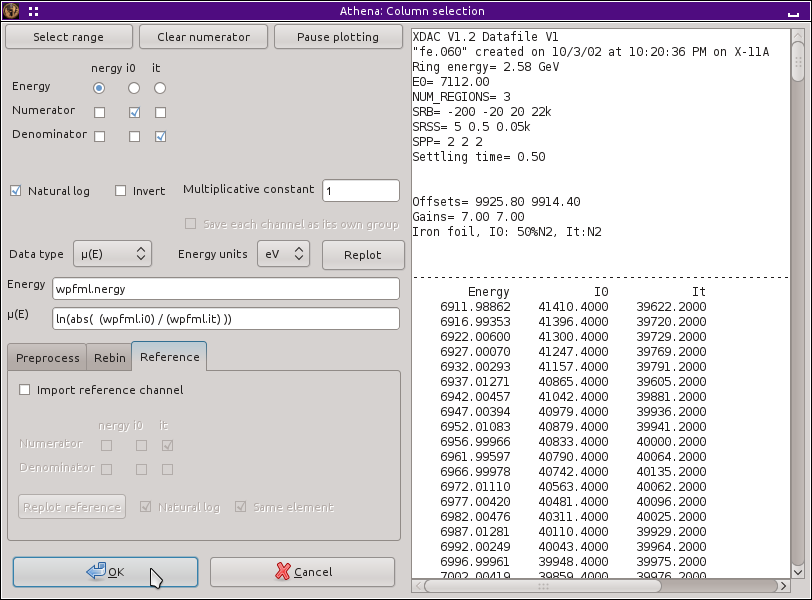
Fig. 12.1 The column selection dialog with columns chosen correctly for the iron foil data.

When I collected these data, I purposefully miscalibrated the monochromator so that I would have a data set for explaining the use of ATHENA's calibration tool. The first thing to do, then, is to correctly calibrate these data.

Open the calibration tool by selecting Calibrate energies from the main menu. The derivative of μ(E) for these data will be plotted, shown below on the left. The choice of edge position, denoted by the little orange circle, is reasonable in that it is close to the first peak of the first derivative, as one expects. The monochromator calibration is obviously wrong as the orange circle is at 7105.5 eV, while the tabulated value for the iron K edge is 7112 eV.

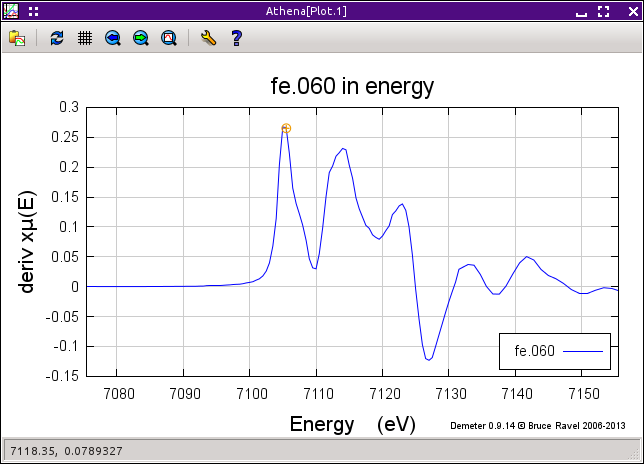
Fig. 12.2 The iron foil data, as plotted in the calibration tool. Derivative of μ(E).

Fig. 12.3 Second derivative of μ(E).

We want to select the peak of the first derivative and set that point to 7112 eV. We can simply use the currently selected point – it is quite close to the peak. Alternately, we can click the Select a point button and try to double-click on the plot, selecting point even closer to the peak. To do that, it would be helpful to change the value of emin and emax in the energy plot tab the replot the data such that a tighter region around the peak is displayed.

A third, highly accurate way of finding the exact peak of the first derivative is to plot the second derivative of the data by selecting second deriv from the display menu. The second derivative of the data along with the currently selected value of edge position are shown on the right of the figure above.

With the second derivative selected for display, the Find zero-crossing button becomes activated. clicking that button will cause ATHENA to search in both directions for the nearest energy value that hits the y=0 axis and select that as the new edge position. The value should be about 7105.3 eV. Click the Calibrate button and return to the main window.

You will notice two things once the main window is displayed again: the value of «E0» is now 7112 and the value of the «eshift» parameter is now about 6.7. In ATHENA, calibration works by simultaneously setting those two parameters such that the selected point has the chosen energy value.

Now, import the second scan at 60K, fe.061. Mark both groups by clicking on their mark buttons and plot them in energy by clicking on the E button.

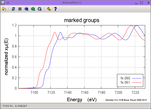
Fig. 12.4 Misaligned iron foil μ(E) data.

Fig. 12.5 The derivatives of the misaligned data, as plotted in the alignment tool.

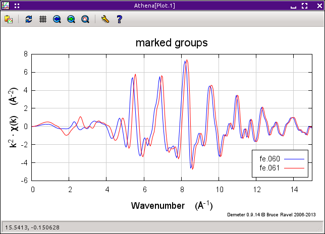
Fig. 12.6 Aligned data plotted in k, but with «E0» unconstrained.

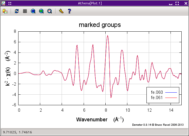
Fig. 12.7 Aligned data plotted in k after constraining «E0». Once aligned and constrained in «E0», these successive scans are quite consistent.

The upper left of the image above shows that these data are not aligned. Since they are successive scans on the same iron foil under the same experimental conditions, we expect these data to be identical within statistical noise. The reason that they are different is that the second scan has not yet been calibrated.

Fixing this requires two steps. First, open the alignment tool by selecting Align scans from the main menu. The two scans are plotted as the derivative of μ(E). The first scan in the list, fe.060, is automatically selected in the Standard menu. The second scan is highlighted in the groups list and is displayed as the Other.

These are very clean data, so the automatic alignment algorithm should work well. Click the Auto align button. If you data is noisy, the automated alignment might not work well, in which case you can use the other buttons to adjust the energy shift until you are satisfied that the data are well aligned.

Returning to the main window, we find that the «eshift» parameter for fe.061 is now about 6.7 eV. When plotted together in energy, the data are well aligned. However when plotted together in k-space by pressing the k button, there remains a problem, as we see in the lower left of the figure above.

The fe.061 data have been aligned, but not calibrated. That is, its «E0» parameter has not been set to the same value as for the fe.060 data. Consequently, the position in the data where k=0 is different for the two spectra and the χ(k) data from the background removal are different.

To correct this, you can either enter the value for «E0» from fe.060 – 7112 eV – into the «E0» text entry box after clicking on fe.061 in the group list. Alternately, you can select fe.060 in the group list, then right click on the «E0» parameter to raise its context menu and select Set all groups to this value of E0. Once the «E0» parameters are set the same for these data sets, we see above in the lower right that the data are quite consistent between these two scans.

Now we need to import the remaining data measured on the iron foil. Using the file selection dialog, select the remaining data files as described in the section on multiple file import and shown below.

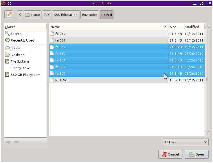
Fig. 12.8 Importing the remaining iron foil data.

Clicking the Open button will import all those data files and list them in the group list. Once they are imported, mark all of the groups either by typing Alt-a or by clicking the A mark button above the group list. Finally select the fe.060 group by clicking on it in the group list. Once you have done all of that, ATHENA will look like this.

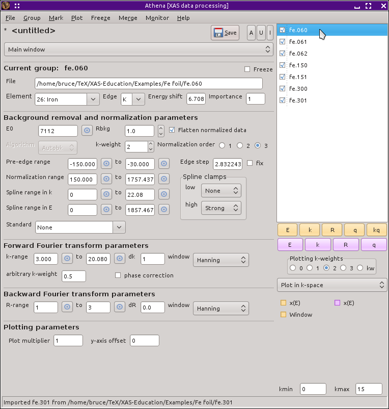
Fig. 12.9 All of the iron foil data have been imported and marked.

At this point, only fe.061 has been aligned to fe.060 and had its value of «E0» properly constrained. We need to do so for the remaining data groups.

Processing all 5 of the remaining data groups would be quite tedious if we had to handle each one individually. Fortunately ATHENA has lots of tools to help process large quantities of data. To align the remaining data to fe.060, choose Align data from the main menu. ATHENA chooses the first item in the group list as the data alignment standard and selects the second group as the one to align. These selections are shown at the top of this.

Of course, fe.061 has already be aligned. If you select any other group by clicking on it in the group list, you will see that it it is not yet aligned. You can align the remaining groups by selecting each on in turn and clicking the Auto align button – but that seems tedious. Much better to click the Align marked groups button. Since all the groups are aligned, the automated alignment algorithm will be applied to each one in turn.

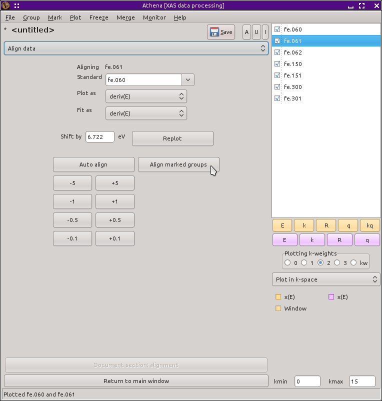
Fig. 12.10 All of the iron foil data are marked and waiting to be aligned.

Once finished, you can click on groups to check on the quality of the alignment. Since these are very good data, the automated alignment should have worked well. Click on the Return to the main window button to continue with the data processing.

Each of the data groups has now been aligned, but only fe.061 has the same value of «E0» as fe.060. Again, clicking through the groups list and editing the «E0» values seems horribly tedious. Here we see the true value of the Set all groups to this value of E0 in the «E0» context menu.

The χ(k) data for the aligned and constrained data are shown below.

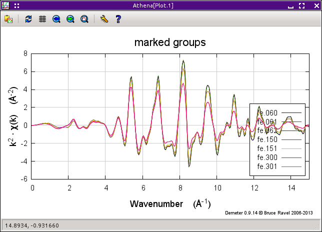
Fig. 12.11 The χ(k) spectra for all the iron foil data.

There is another, perhaps quicker, way of doing everything that is described above. To start, import the fe.060 data and calibrate it as explained at the start of this section. Then use the file selection dialog to select all of the remaining data. Click to the Preprocess tab, select the fe.060 data as the standard, then click the Mark, Align, and Set parameters checkbuttons.

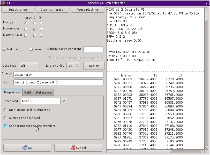
Fig. 12.12 Using the preprocessing features of the column selection dialog to align and constrain data on the fly as it is imported.

Now click the Open button. As the remaining data are imported, the alignment and «E0» constraint will happen on the fly and the new group will be marked. Once the file selection dialog using these preprocessing features is finished, ATHENA should look just like it did in the screenshot above.

As a final chore in this section, we will merge the data measured at each temperature. Since the data are properly aligned and calibrated, this is a fine time to perform the merge. First mark each data group that should be merged together. As we see in the screenshot below, the two groups measured at 300K are marked. Select Merge ‣ Merge mu(E). This will perform the merge then insert a new group in the group list. Then select Group ‣ Rename current group, type Alt-l, or double-click on the group list entry to give the merged group a more suggestive name. Repeat this process for the data at each temperature.

Now you are ready to begin analysis on the iron foil data!

Fig. 12.13 Merging the data at each temperature and renaming the merged groups.

---

DEMETER is copyright © 2009-2016 Bruce Ravel – This document is copyright © 2016 Bruce Ravel

This document is licensed under The Creative Commons Attribution-ShareAlike License.

If DEMETER and this document are useful to you, please consider supporting The Creative Commons.